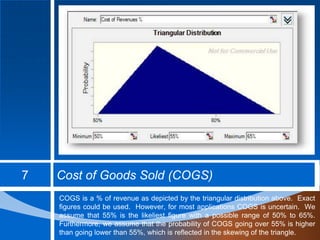
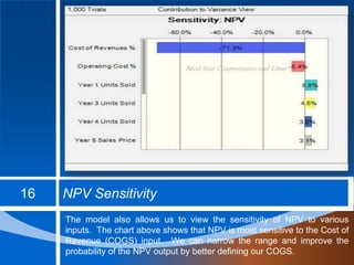
Intellectual Property (IP) Licensing Valuation ModelBy: Mark West1
Valuation Model SummaryThe Intellectual Property Licensing Valuation Model is based on the Monte Carlo simulation and was created using Crystal Ball software.  The model provides an Internal Rate of Return (IRR) and Net Present Value (NPV) valuation while taking into account the inherently high uncertainty (risk) of cost and revenue associated with embryonic technology projects.  The widget and its associated cost/revenue figures are fictitious.  However, the model can be applied to real world projects.2
The model is shown above.  Inputs to the model are highlighted bright green.  Forecast outputs are highlighted light blue.  For the sake of the presentation, sample cost and revenue ranges have been chosen.Intellectual Property Licensing Valuation Model3
Sales Price AssumptionsThe sales price of the widget is uncertain.  However, lets assume that the likeliest price is $100.  Also, we are confident that the price will not be lower than $90 or higher than $110.  For this reason the triangular distribution, shown on the following slide, has been chosen.  The probability diminishes as the price approaches $90 and $110, respectively.  Outside of these boundaries the probability is zero.  These same parameters have been used for all five years of sales (see slide 3).  However, the model allows complete flexibility for every year of data.  For example, we could say that in year two the likeliest price is $150 with boundaries of $125 and $175.  Also, we could use a rectangular distribution if we felt that every level of price was equally likely.4
Triangular Sales Distribution5
Units sold in year one is assumed to be 50,000 units, with an additional increase in units sold of 50,000 per year.  However, because of the uncertainty of sales we assume a normal probability distribution,  with a standard deviation of 10,000 units (pictured above).  For example, it is 68.2% likely that the units sold in the first year will be between 40,000 and 60,000.Units Sold6
COGS is a % of revenue as depicted by the triangular distribution above.  Exact figures could be used.  However, for most applications COGS is uncertain.  We assume that 55% is the likeliest figure with a possible range of 50% to 65%.  Furthermore, we assume that the probability of COGS going over 55% is higher than going lower than 55%, which is reflected in the skewing of the triangle.Cost of Goods Sold (COGS)7
Operating Costs are assumed to be a % of Gross Income using the normal distribution above.  In this case we assume a mean Operating Cost of 15% with a standard deviation of 2%.Operating Costs8
Valuation Model OutputWith all of the inputs defined we are ready to run the Monte Carlo simulation.  The model runs 5,000 trials utilizing the data input from the previous slides, generating 59,780 random data inputs within the probabilities and ranges we have defined.  The entire simulation is complete in 0.4 seconds.9
As shown on slide 3, one of the forecasted outputs is Net Income.  The chart above displays the Net Income forecast for years 1 – 5 within the Certainty Bands (10%, 25%, 50%, 90%) defined by the chart legend.  The Certainty Bands can be customized for each valuation.Net Income10
Internal Rate of Return (IRR)The forecasted range and corresponding frequency/probability of Internal Rate of Return (IRR) is given in the chart on the following slide.  The values were generated based on the 5,000 trials run by the model.  The model also provides the following useful statistics.Trials:		5,000Mean:		70%Median:		70%Standard Deviation:	6%Skewness:		-0.0221Kurtosis:		2.80Coeff. of Variability:	0.0866Minimum:		53%Maximum:		92%Mean Std. Error:	0%11
IRR Chart12
The model allows us to view the sensitivity of IRR to various inputs.  The chart above shows that IRR is most sensitive to the Cost of Revenue (COGS) and units sold in year one.  We can improve the probability of our model by better defining our COGS and sales.Internal Rate of Return (IRR) Sensitivity13
Net Present Value (NPV)The forecasted range and corresponding frequency/probability of NPV is given in the chart on following slide. In theory, at NPV = 0 the licensee would be equally willing to accept or reject the project.  However, in practice most companies have a hurdle rate (%) which exceeds the company Weighted Average Cost of Capital (WACC) or “discount rate”.  Slide 11 shows the same chart using an assumed hurdle rate (20%).  The NPV statistics are as follows.Trials:		5,000Mean:		$9,946,425Median:		$9,985,205Standard Deviation:	$1,132,167Skewness:		-0.0600Kurtosis:		2.61Coeff. of Variability:	0.1138Minimum:		$6,162,910Maximum:		$13,342,820Mean Std. Error:	$16,01114
NPV Probabilities15
The model also allows us to view the sensitivity of NPV to various inputs.  The chart above shows that NPV is most sensitive to the Cost of Revenue (COGS) input.  We can narrow the range and improve the probability of the NPV output by better defining our COGS.NPV Sensitivity16
Hurdle Rate NPVThe simulation was run again using an assumed hurdle rate of 20% as our discount rate.  At a minimum, we should expect a royalty payment of $4,117,984, either paid upfront “paid-up” or via a stream of payments that are tied to revenue and equivalent in NPV terms.The model also allows us to view NPV within customized ranges of certainty.  For example, based on the chart on the following slide, we can be 80% certain that the NPV of the project will be greater than $5,764,874.  Using the 80% figure, we might be able to persuade a potential licensee that a royalty payment of $5,764,874 is equitable.  After all, 80% is a high level of confidence.17
Hurdle Rate NPV Chart18

Intellectual Property Licensing Valuation Model

  • 1.
    Intellectual Property (IP)Licensing Valuation ModelBy: Mark West1
  • 2.
    Valuation Model SummaryTheIntellectual Property Licensing Valuation Model is based on the Monte Carlo simulation and was created using Crystal Ball software. The model provides an Internal Rate of Return (IRR) and Net Present Value (NPV) valuation while taking into account the inherently high uncertainty (risk) of cost and revenue associated with embryonic technology projects. The widget and its associated cost/revenue figures are fictitious. However, the model can be applied to real world projects.2
  • 3.
    The model isshown above. Inputs to the model are highlighted bright green. Forecast outputs are highlighted light blue. For the sake of the presentation, sample cost and revenue ranges have been chosen.Intellectual Property Licensing Valuation Model3
  • 4.
    Sales Price AssumptionsThesales price of the widget is uncertain. However, lets assume that the likeliest price is $100. Also, we are confident that the price will not be lower than $90 or higher than $110. For this reason the triangular distribution, shown on the following slide, has been chosen. The probability diminishes as the price approaches $90 and $110, respectively. Outside of these boundaries the probability is zero. These same parameters have been used for all five years of sales (see slide 3). However, the model allows complete flexibility for every year of data. For example, we could say that in year two the likeliest price is $150 with boundaries of $125 and $175. Also, we could use a rectangular distribution if we felt that every level of price was equally likely.4
  • 5.
  • 6.
    Units sold inyear one is assumed to be 50,000 units, with an additional increase in units sold of 50,000 per year. However, because of the uncertainty of sales we assume a normal probability distribution, with a standard deviation of 10,000 units (pictured above). For example, it is 68.2% likely that the units sold in the first year will be between 40,000 and 60,000.Units Sold6
  • 7.
    COGS is a% of revenue as depicted by the triangular distribution above. Exact figures could be used. However, for most applications COGS is uncertain. We assume that 55% is the likeliest figure with a possible range of 50% to 65%. Furthermore, we assume that the probability of COGS going over 55% is higher than going lower than 55%, which is reflected in the skewing of the triangle.Cost of Goods Sold (COGS)7
  • 8.
    Operating Costs areassumed to be a % of Gross Income using the normal distribution above. In this case we assume a mean Operating Cost of 15% with a standard deviation of 2%.Operating Costs8
  • 9.
    Valuation Model OutputWithall of the inputs defined we are ready to run the Monte Carlo simulation. The model runs 5,000 trials utilizing the data input from the previous slides, generating 59,780 random data inputs within the probabilities and ranges we have defined. The entire simulation is complete in 0.4 seconds.9
  • 10.
    As shown onslide 3, one of the forecasted outputs is Net Income. The chart above displays the Net Income forecast for years 1 – 5 within the Certainty Bands (10%, 25%, 50%, 90%) defined by the chart legend. The Certainty Bands can be customized for each valuation.Net Income10
  • 11.
    Internal Rate ofReturn (IRR)The forecasted range and corresponding frequency/probability of Internal Rate of Return (IRR) is given in the chart on the following slide. The values were generated based on the 5,000 trials run by the model. The model also provides the following useful statistics.Trials: 5,000Mean: 70%Median: 70%Standard Deviation: 6%Skewness: -0.0221Kurtosis: 2.80Coeff. of Variability: 0.0866Minimum: 53%Maximum: 92%Mean Std. Error: 0%11
  • 12.
  • 13.
    The model allowsus to view the sensitivity of IRR to various inputs. The chart above shows that IRR is most sensitive to the Cost of Revenue (COGS) and units sold in year one. We can improve the probability of our model by better defining our COGS and sales.Internal Rate of Return (IRR) Sensitivity13
  • 14.
    Net Present Value(NPV)The forecasted range and corresponding frequency/probability of NPV is given in the chart on following slide. In theory, at NPV = 0 the licensee would be equally willing to accept or reject the project. However, in practice most companies have a hurdle rate (%) which exceeds the company Weighted Average Cost of Capital (WACC) or “discount rate”. Slide 11 shows the same chart using an assumed hurdle rate (20%). The NPV statistics are as follows.Trials: 5,000Mean: $9,946,425Median: $9,985,205Standard Deviation: $1,132,167Skewness: -0.0600Kurtosis: 2.61Coeff. of Variability: 0.1138Minimum: $6,162,910Maximum: $13,342,820Mean Std. Error: $16,01114
  • 15.
  • 16.
    The model alsoallows us to view the sensitivity of NPV to various inputs. The chart above shows that NPV is most sensitive to the Cost of Revenue (COGS) input. We can narrow the range and improve the probability of the NPV output by better defining our COGS.NPV Sensitivity16
  • 17.
    Hurdle Rate NPVThesimulation was run again using an assumed hurdle rate of 20% as our discount rate. At a minimum, we should expect a royalty payment of $4,117,984, either paid upfront “paid-up” or via a stream of payments that are tied to revenue and equivalent in NPV terms.The model also allows us to view NPV within customized ranges of certainty. For example, based on the chart on the following slide, we can be 80% certain that the NPV of the project will be greater than $5,764,874. Using the 80% figure, we might be able to persuade a potential licensee that a royalty payment of $5,764,874 is equitable. After all, 80% is a high level of confidence.17
  • 18.