F5 Revision D08

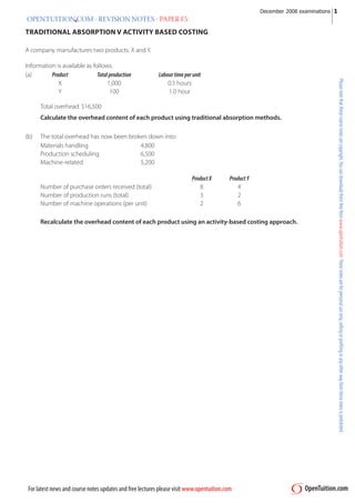
TRADITIONAL ABSORPTION V ACTIVITY BASED COSTING
A company manufactures two products: X and Y.
Information is available as follows:
(a) Product Totalproduction Labourtimeperunit
X 1,000 0.5 hours
Y 100 1.0 hour
Total overhead: $16,500
Calculate the overhead content of each product using traditional absorption methods.
(b) The total overhead has now been broken down into:
Materials handling 4,800
Production scheduling 6,500
Machine-related 5,200
ProductX ProductY
Number of purchase orders received (total) 8 4
Number of production runs (total) 3 2
Number of machine operations (per unit) 2 6
Recalculate the overhead content of each product using an activity-based costing approach.
For latest news and course notes updates and free lectures please visit www.opentuition.com
1
OPENTUITION.COM - REVISION NOTES - PAPER F5
December 2008 examinations

ACTIVITY BASED COSTING
* Gives fairer valuation of cost per unit
• Identifies cost driver for each overhead rather than absorb all at one arbitrary rate
* Focuses attention on cost drivers
• Leads to better control of overheads
BUT:
* time - consuming to identify cost drivers
* not always possible to identify a cost driver
2

THROUGHPUT ACCOUNTING
A company produces 3 products, details of which are given below:
A B C
Selling price 50 60 40
Materials 10 15 8
Labour 10 5 6
Variable overheads 18 20 4
Fixed overheads 5 8 10
43 48 28
Profit p.u. 7 12 12
Machine hours p.u. 1 hr 2 hrs 2 hrs
Maximum demand 500u 500u 500u
The machine time is limited to 1,800 hours.
Determine the optimum production plan and calculate the maximum profit
(a) using key factor analysis
(b) using throughput accounting
Main assumptions of throughput accounting:
* in the short term, all costs except materials are fixed
* inventory levels are kept to a minimum, ideally zero.
3

LIFE CYCLE COSTING
Consider costs and revenues over the estimated entire life of a product.
Phases of life cycle:
* Development
* Introduction
* Growth
* Maturity
* Decline
For example, might plan to have high selling price initially (high development/introduction costs, low competition),
and then to have lower prices during the maturity phase (higher volume of sales, lower costs, more competition) and
plan for eventual withdrawal of product (and replacement with new product) towards end of life cycle.
4

TARGET COSTING
1. Determine a realistic / competitive selling price.
2. Determine the profit required (e.g. required profit margin)
3. Calculate the maximum cost p.u. in order to achieve the required profit.
4. This is the target cost
5. Compare the estimated actual cost with the target cost. If higher, look for ways of achieving the target cost.
5

JUST-IN-TIME INVENTORY MANAGEMENT
The objective is to remove the need to keep inventory.
The main steps in order to achieve this are:
* total quality management
if there is no waste or damage to materials, there is less need for stock
if all finished goods are‘perfect’there is less need for stock
* fast production
the faster the production the less work-in-progress
goods can be produced to order, rather than being produced for stock
* frequent, guaranteed deliveries of raw materials
it is the supplier who then has to keep stock, rather than the company
6

PRICING
Full cost plus:
Take full cost (i.e. including fixed overheads) and add on a percentage
Example
variable cost of production $5 p.u.
budgeted fixed costs $60,000 p.a.
budgeted production 20,000 units p.a.
mark-up of 30%
fixed costs p.u. = 60,000/20,000 = $3
full cost = 5 + 3 = $8 p.u.
selling price = $8 + 30% x $8 = $10.40 p.u.
Ensures that company covers fixed costs, BUT how to budget the level of production?
Takes no account of the effect of the selling price on demand.
Marginal cost plus:
Take marginal (variable cost) and add on a percentage
Example
Variable cost of production $5 p.u.
budgeted fixed costs $60,000 p.a.
budgeted production 20,000 units p.a.
mark-up of 50%
marginal cost = $5 p.u.
selling price = $5 + 50% x $5 = $7.50 p.u.
Avoids the problems of absorbing fixed overheads, BUT what percentage to add in order to ensure that fixed overheads
are covered?
Takes no account of the effect of the selling price on demand.
7

THEORETICAL PRICING
1. At a selling price of $80 p.u., the demand will be 50,000 units p.a..
For every $5 change in the selling price, the demand will change by 2,000 units.
Derive the price/demand equation.
2. At a selling price of $100 p.u., the demand will be 80,000 units p.a..
For every $10 change in the selling price, the demand will change by 5,000 units.
Derive the price/demand equation.
3. At a selling price of $200, the demand will be 100,000 units p.a..
The demand will change by 10,000 units for every $30 change in the selling price.
The marginal revenue is given by: MR = 500 – 0.006Q
The total costs will be 60,000 + 8Q
What should be the selling price p.u. to achieve maximum profit p.a.?
8

RELEVANT COSTING
* Suitable for one-off contracts.
* Calculate the future, incremental (i.e. extra), cash flows which will result from doing the contract.
Sunk costs: costs already incurred - not relevant
Opportunity costs: lost income as a result of doing the contract - are relevant
Fixed costs: only relevant if the total changes as a result of doing the contract
Examples:
1. Contract requires 200 kg of material X.
Company has 500 kg in stock, which originally cost $6 per kg..
Material X has no other use, and if not used in the contract will be scrapped for $2 per kg..
2. Contract requires 300 kg of material Y.
Company has 600 kg in stock, which originally cost $10 per kg..
Material Y is in regular use by the company has the current purchase price is $12 per kg..
3. Contract requires 50 hours of skilled labour.
The company pays skilled labour $5 per hour, and there is currently plenty of idle time.
Labour is paid $5 per hour.
There is no spare time, and the contract would have to be done in overtime.
Overtime is paid at normal rate plus 50%.
Labour is paid $5 per hour.
Labour is currently fully occupied making another product which is generating a contribution of $8 p.u.
Each unit of the other product requires 2 hours of skilled labour.
9

UNCERTAINTY
Sales per week
Sales(units) Probability
10 0.3
20 0.5
30 0.2
Selling price: $20 p.u.
Cost: $10 p.u.
Any unsold units must be sold as scrap for $1 p.u.
The company can contract to purchase 10, 20 or 30 units each week.
How many units should they contract for?
(a) Expected Values
(b) Maximax
(c) Maximin
(d) Minimax Regret
10

BUDGETING (1)
Incremental budgeting
Take last years figures and adjust for growth and inflation.
Easiest and most common approach, but assumes that we continue to do things the same way. (For example, if we
make our products by hand, we will budget to continue to make them by hand and ignore the fact that maybe there
are now machines capable of producing them.)
Zero based budgeting
Ignore what currently happens.
Instead, identify different solutions available, cost them out, and budget on adopting the best solution.
For example, if our product can be made by hand or made by machine, then cost out both approaches, see which is the
cheaper, and budget on that basis.
Although zero based is in principle a much better approach, it is time-consuming and requires expertise.
A realistic way of using a zero based approach is to apply it to one area of the business each year, and budget the other
areas using an incremental approach.
Activity based budgeting
Use an activity based costing approach. Budget the costs for each activity and how each activity is being used, in an
attempt to ensure that each activity is being used efficiently.
11

BUDGETING (2)
Top-down budgeting
Budget is prepared centrally and then imposed on the managers of each department
Bottom-up budgeting
Each manager produces his/her budget. It is the job of central management to make sure the budgets are challenged
and that different departments budgets coordinate with each other.
Bottom-up budgeting is regarded as being more motivational for managers. However the budgets do need to be
challenged well otherwise there is the danger of managers introducing slack into their budgets.
12

BUDGETING (3)
Fixed budget – The original budget based on the originally estimated levels of sales and production.
The original budget profit remains the overall target of the company.
Flexed budget – The budget is adjusted (or flexed) for the actual levels of sales and production. This
is usually done monthly and is used for the purpose of control (compare the actual
results with the flexed budget. i.e. variance analysis)
Rolling budget
(continuous budgeting)
– Update the budget each month and always have a budget for the next 12 months
13

FORECASTING
HIGH LOW METHOD
Month Sales
(units)
1 23100
2 24000
3 24100
4 24800
5 25000
6 26030
7 26000
8 27100
9 27200
10 27800
11 27800
12 27500
Month Units
High 12 27500
Low 1 23100
Difference 11 4400
Change per month: 4400 / 11 = 400
Forecast for next month: 27500 + 400 = 27900 units
14

FORECASTING
REGRESSION
x y xy x2
Month Sales(units)
1 23100 23100 1
2 24000 48000 4
3 24100 72300 9
4 24800 99200 16
5 25000 125000 25
6 26030 156180 36
7 26000 182000 49
8 27100 216800 64
9 27200 244800 81
10 27800 278000 100
11 27800 305800 121
12 27500 330000 144
Σx = 78 Σy = 310430 Σxy = 2081180 Σ x2
= 650
n = number of pairs of observations = 12
b =
nΣxy – ΣxΣy
=
12 x 2081180 – 78 x 310430
=
760620
= 443.25
nΣx2
– (Σx)2
12 x 650 – 78 x 78 1716
a =
Σy
–
bΣx
=
310430
–
443.25 x 78
= 22988
n n 12 12
y = 22988 + 443.25x
Forecast for month 13 = 22988 + 443.25 x 13 = 28750 units
15

FORECASTING
TIME SERIES
Sales(units) MovingAverage CentredAverage SeasonalVariation SeasonalVariation
(Additive) (Multiplicative)
2005 – qtr 1 1200
2005 – qtr 2 1100
2005 – qtr 3 1250
2005 – qtr 4 1000
2006 – qtr 1 1300
2006 – qtr 2 1180
2006 – qtr 3 1340
2006 – qtr 4 1110
2007 – qtr 1 1410
2007 – qtr 2 1290
2007 – qtr 3 1450
2007 – qtr 4 1200
16

LEARNING CURVES
As cumulative output doubles, the cumulative average time (labour cost) per unit falls to a fixed percentage of the
previous average time (labour cost)
Example 1
First batch takes 100 hours to produce. There is a 75% learning effect.
How long will it take to produce another 7 batches.
Example 2
First batch takes 60 hours to produce. There is an 80% learning effect.
How long will it take to produce the 7th
batch?
Learning curve formula: y = axb
y = average time per batch
a = time for initial batch
x = number of batches
b = learning factor
b =
log r
log 2
17

OPERATING STATEMENT (ABSORPTION COSTING)
Original Budget Profit
Sales Volume Variance
units
Actual sales
Budgeted sales
units × Standard profit p.u.
Sales Price Variance
Actual sales at actual S.P.
Actual sales at standard S.P
Materials Expenditure Variance
Actual purchases at actual cost
Actual purchases at standard cost
Materials Usage Variance
kg
Actual usage
Standard usage for actual production
kg × Standard cost
Labour Rate of Pay Variance
Actual hours paid at actual cost
Actual hours paid at standard cost
Labour Idle Time Variance
hours
Actual hours paid
Actual hours worked
× Standard cost
Labour Efficiency Variance
hours
Actual hours worked
Standard hours for actual production
× Standard cost
Variable Expenditure Variance
Actual hours worked at actual cost
Actual hours worked at standard cost
Variable Efficiency Variance
hours
Actual hours worked
× Standard cost
Fixed Overhead Expenditure Variance
Actual total
Budget Total
Fixed Overhead Volume Variance
units
Actual production
Budget production
× Standard cost per unit
Actual Profit
18

OPERATING STATEMENT (MARGINAL COSTING)
Original Budget Profit
Sales Volume Variance
units
Actual sales
Budget sales
units × Standard contribution p.u.
Sales Price Variance
Actual sales at actual S.P.
Actual sales at standard S.P
Materials Expenditure Variance
Actual purchases at actual cost
Actual purchases at standard cost
Materials Usage Variance
kg
Actual usage
Standard usage for actual production
kg × Standard cost
Labour Rate of Pay Variance
Actual hours paid at actual cost
Actual hours paid at standard cost
Labour Idle Time Variance
hours
Actual hours paid
Actual hours worked
× Standard cost
Labour Efficiency Variance
hours
Actual hours worked
× Standard cost
Variable Expenditure Variance
Actual hours worked at actual cost
Actual hours worked at standard cost
Variable Efficiency Variance
hours
Actual hours worked
× Standard cost
Fixed Overhead Expenditure Variance
Actual total
Budget Total
Actual Profit
19

VARIANCE ANALYSIS
Budget sales and production of Product X are 600,000 units p.a. at a standard selling price of $100 p.u.
The original standard costs of production were:
Materials: 2 kg @ $20 per kg
Labour: 1.5 hrs @ $2 per hr
Variable overheads: 1.5 hrs @ $6 per hr
Fixed overheads were budgeted at $10.8M for the year.
Since preparation of the budget, the suppliers of the materials had announced a permanent price increase of 10%.
As a result the manufacturing process was examined and ways were found of reducing material usage by 5% without
affecting the quality of finished goods.
Actual results for January were as follows:
Sales: 53,000 units @ $95 p.u.
Production costs for 55,000 units produced:
Materials (110,000 kg) $2,300,000
Labour (85,000 hrs) $180,000
Variable Overheads $502,000
Fixed Overheads $935,000
Prepare an operating statement.
(Note: the company’s policy is to use marginal costing)
20

VARIANCES
1. Always marginal costing in exam unless told otherwise, but check carefully.
2. Always show standard cost per unit (cost card) unless given in question. (Make sure you still get the marks even
if you have misread something).
3. Examiner sometimes uses the word ‘cost variance’ to mean ‘total variance’. (e.g. ‘calculate for materials the cost,
expenditure, and usage variances’. Means expenditure and usage as normal + total variance. Do not calculate total
separately, it is simply the total of expenditure + usage).
4. If more than one material, do NOT calculate mix yield variances unless asked for. (or unless he says‘the materials
are substitutable’but he is unlikely to use these words).
5. Remember: for cost variances we are always comparing actual costs with standard cost for actual level of
production. It is worth writing down the actual level of production if you have misread, it is then obvious what
you were trying to do.
6. Planning and Operational Variances
(a) Planning (or Revision) Variance
• This is the difference between original budget profit and revised budget profit, due to permanent
changes.
• This variance cannot be ‘corrected’ (or controlled) but when it is identified that it is going to occur
company may decide to change plans for the future ie. feed-forward control.
(b) Operational Variances
• These are differences between actual results and revised budget.
• Normally calculated monthly. It is too late to do anything about the period under review, but can use
information to attempt to correct (or control) any problems for the future. ie. feedback control.
21

FIXED OVERHEAD VARIANCES
A company uses absorption costing.
The standard cost card is as follows:
Materials (2 kg at $30 per kg) 60.00
Labour ( 4 hours at $5 per hour) 20.00
Fixed overheads (4 hours at $4 per hour) 16.00
$96.00
Standard selling price $120.00
Budget production and sales: 50,000 units
Actual production and sales: 60,000 units
All sales were made at the standard selling price, and materials usage and cost were as per the standard cost card.
230,000 labour hours were paid and worked, at a cost of $ 1,150,000
Actual expenditure on fixed overheads was $ 1,000,000
22

LABOUR VARIANCES - EXCESS IDLE TIME
The standard costs of labour are as follows:
5 hours (paid) at $3.60 per hour = $18 p.u.
It is budgeted that there will be 10% idle time.
The actual production is 10,000 units and the actual labour costs are as follows:
$185,000 was paid for 48,000 hours, of which 46,000 were actually worked.
23

MIX YIELD VARIANCES
Standard cost per unit of output:
A 6 kg @ $8 48
B 2 kg @ $4 8
56
Actual results:
Materials input A 99,000 kg at a total cost of $800,000
B 36,000 kg at a total cost of $140,000
Actual production: 16,000 units
24

MIX YIELD - ANSWER
EXPENDITURE/PRICE
Actual
purchases
@ Actualcost
Actual
purchases
@ Standardcost
kg $ kg $
A 99,000 800,000 99,000 $8 $792,000
B 36,000 140,000 36,000 $4 144,000
135,000 $940,000 135,000 $936,000
$4,000 (A)
MIX
Actualusage @ Standardcost
Stdmixforactual
totalinput
@
Standard
cost
kg $ kg $
A 99000 792,000 (6/8) 101,250 $8 810,000
B 36000 144,000 (2/8) 33,750 $4 135,000
135,000 $936,000 135,000 $945,000
$9,000 (F)
YIELD
Stdmixforactual
totalinput
@ Standardcost @ Stdmixforfinal
production
Standardcost
kg $ kg $
A 101,250 810,000 (6/8) 96,000 $8 768,000
B 33,750 135,000 (2/8) 32,000 $4 128,000
135,000 $945,000 128,000 $896,000
16,000 @ 8kg
$49,000 (A)
SUMMARY:
EXP 4,000 (A) 44,000 (A)
MIX 9,000 (F) (TOTAL)
40,000 (A)
YIELD 49,000 (A) usage
25

PERFORMANCE INDICATORS
RETURN ON CAPITAL
Profit before interest tax
× 100%
Long term capital
GEARING
Long term debt
or
Long term debt
Equity Equity + Long term debt
INTEREST COVER
Profit before interest tax
Interest
OPERATING PROFIT MARGIN
Operating Profit
× 100%
Sales
CURRENT RATIO
Current Assets
Current liabilities
QUICK RATIO
Current Assets – Stock
Current liabilities
EARNINGS PER SHARE (E.P.S.)
Profit after interest tax
Number of shares
P / E ratio
Market value per share
Earnings per share
26

RETURN ON INVESTMENT V RESIDUAL INCOME
Division X of Y plc is currently reporting profits of $100,000 p.a. on capital employed of $800,000
A new project is being considered which will cost $100,000 and is expected to generate profits of $15,000 p.a.
The Cost of Capital of Y plc is 16%
(a) Should Y plc accept or reject the project?
(b) Will the manager of Division X be motivated to accept the project if his performance is measured
(i) on Return on Investment?
(ii) on Residual Income?
27

DIVISIONAL PERFORMANCE MEASUREMENT
Type of responsibility centre:
Cost centre:
Manager has authority for decisions over costs (but not revenue)
Revenue centre:
Manager has authority for decisions over revenue (but not costs)
Profit centre:
Manager has authority for decisions over costs and revenues (but not capital investment decisions)
Investment centre:
Manager has authority for decisions over costs, revenues, and new capital investment.
Controllable factors:
The manager should only be assessed over those items over which he has control.
For example, if a manager is given authority to make decisions over everything except salary increases which are
dictated by central management, then it would be unfair to include salaries in his performance measurement.
If (for example) it is a profit centre, then for the purposes of measuring his performance the profit of the division should
be calculated ignoring salaries.
28

TRANSFER PRICING
OBJECTIVES:
* Goal congruence
* Performance appraisal
* Divisional autonomy
OVERALL:
* Must maximise group profit
PRACTICAL:
* T.P. often fixed by Head Office
* Problem – loss of autonomy
– possibility of dysfunctional decisions
APPROACH:
Allow individual managers to negotiate the transfer price
Selling division:
Minimum T.P. = Marginal cost + opportunity cost
Receiving division:
Maximum T.P. is lower of
(a) external purchase price (on intermediate market)
and
(b) net marginal revenue (selling price less costs of receiving division)
29

TRANSFER PRICING
[S = selling division; R= receiving division]
S R
1. Variable production cost 15 8
Final selling price $30
2. As (1), but intermediate market exists.
S can sell intermediate market at $18; R can buy on intermediate market at $20
(a) S has unlimited production capacity and there is limited demand on the intermediate
market
(b) S has limited production capacity and there is unlimited demand on the intermediate
market
3. S has restricted capacity to make A and B
R wants product A.
A B
S’s Variable production cost per unit 80 120
S’s Intermediate market price per unit 100 150
30

NON-FINANCIAL PERFORMANCE MEASURES
Quality
Flexibility
Efficiency (Resource utilisation)
Innovation
Competitiveness
31

BACKFLUSH COSTING
Traditional costing systems use sequential tracking of costs which means that means that costing is synchronised
with the physical sequences of production: purchase, work-in-progress, finished goods. In a system where there were
several stages of production, this approach led to very complex accounting as costs were gradually built up in a unit as
it progressed.
Traditional costing:
WIPstage1 WIPstage2 Finishedgoods
Materialsaccount
Costs in Costs out
to WIP
Conversioncosts
Costs in Costs out
to WIP
Material
To cost
of sales
In just-in-time manufacturing environments, work-in-progress should be very low and the effort spent carefully costing
each stage of production might not be worthwhile.
Backflush costing does not attempt to value work-in progress (other than material content) and this can greatly
simplify accounting. Typically, material costs and conversion costs are initially debited to appropriate accounts then
are transferred straight to finished goods as these are produced. Backflush costing is sometimes called‘delayed costing’
which is a more informative name.‘Trigger points’refer to where inventory costing take place. In the following example
there are two trigger points:
1 The purchase of materials
2 Production of finished goods.
There are only two sorts of inventory – raw materials and finished goods. Costs are transferred only when finished
goods are produced. WIP is not separately valued.
Finishedgoods
Materialsaccount
Costs in Costs out
to finished
goods
Conversioncosts
Costs in Costs out
to WIP
Material
To cost
of sales
32

FIXED OVERHEAD VARIANCES - ABSORPTION COSTING
Total Variance
Actual total fixed overheads
Standard cost for actual production
Analysis of Total Variance
Expenditure Variance
Actual Total
Budget Total
Volume Variance
units
Actual Production
Budget Production
× Standard cost per unit =
Analysis of Volume Variance
Capacity Variance
hours
Actual hours worked
Budget hours
× Standard cost per hour =
Efficiency Variance
hours
Actual hours worked
× Standard cost per hour =
Summary
Expenditure Variance
Capacity Variance
Efficiency Variance
Note: Analysis Volume Variance into capacity and efficiency variances assumes that budget production was limited by
labour hours available. Therefore we can only produce more than budget if
a) we have more hours available (capacity)
and/or
b) workers work faster (efficiency)
33

VARIANCES - DIFFERENCES BETWEEN MARGINAL AND ABSORPTION COSTING
All the variances are the same in both cases, except:
Sales Volume Variance:
Take difference in units between budget and actual sales, and cost out at:
Marginal costing: Standard contribution per unit
Absorption costing: Standard profit per unit
Fixed Overheads Variances
Marginal costing: Only expenditure variance
Absorption costing: Expenditure variance and volume variance
(Volume Variance can be analysed into
capacity and efficiency - see separate sheet)
34

56 student accountant May 2008
technical
The transition from Paper F2 (and the
previous paper, Paper 1.2) to Paper F5 cannot
be underestimated. When preparing for the
Paper F5 exam, students need to carefully
consider what the examiner is looking for.
The purpose of this article is to point students
in the right direction when studying the
interpretation of financial data – which is a
major topic in the Paper F5 syllabus.
This article has been written following
marking of the December 2007 exam papers.
Although there were many very good answers
to Question 2 (‘Ties Only’), it was clear that
more guidance is needed for some candidates.
Students are advised to look at Question 2
while reading this article, as extracts from
the question are used to illustrate points and
explain the techniques needed.
Assessing FinAnciAl PerForMAnce
In the December 2007 exam, candidates were
asked to assess the financial performance of
the business in its first two quarters, when
sales had jumped 61% from Quarter 1 to
Quarter 2. This calculation should present
no problem ((Q2/Q1)-1) expressed as a %
increase). However, an ‘assessment’ requires
a qualitative comment or two. A percentage
alone will not gain a pass mark.
In most questions there will be some
background information – you should use
it. Ties Only operated in a competitive
environment – as stated in the question – and
so a 61% increase in one quarter sounds
pretty good in a competitive situation, and to
say so will earn a mark. It was also the first
two quarters of the business year and so this
level of growth is impressive – another mark.
If you then go on to say that such high growth
rates are often hard to maintain, you will gain
another mark. Top-scoring students should be
aiming to make these kinds of observations.
Hypothesising as to why the growth is
analyse thishappening is also a source of marks. Revenue
growth can be the result of extra volume or
increasing prices. In the case of Ties Only, it is
much more likely to be increased volume; the
price will surely be constrained by competition,
and from the information provided in Part (b),
you can work out that prices are falling
(although that calculation was not required).
Suggesting that Ties Only has secured more
customers, and hence increased volume of
sales, scored a mark.
Candidates must be brave and commit
themselves. You must express an opinion. It
is not acceptable to suggest that management
investigate. Although in the real world this
may well happen, in the exam hall you have to
demonstrate that you know where to look.
inTerPreTATion
The principle of interpretation can be applied
to other areas of the syllabus. In Question 3
of the December 2007 exam, candidates
were required to interpret sales performance.
Again, it is recommended that you refer to
Question 3. Broadly, in this question, the
market was shrinking and the company was
struggling a little as a result. It had reduced
sales prices and fought off an 11% fall in the
market, losing only 2% of its budgeted sales.
This is a good performance, taking the falling
market into consideration.
I would expect candidates to be able
to interpret the variances and reach the
above conclusions. So, if you are given the
following information:
sales price variance $105,600 adv
sales volume variance $28,000 adv
sales market size variance $140,000 adv
sales market share variance $112,000 fav
You should be able to hypothesise as to what
has happened, using the information given in
the question and your understanding of the
data. Adverse sales price variance must mean
that sales prices have fallen. This could be the
result of competitive pressure. Adverse sales
volume variance means that the business
hasn’t achieved its budget, which is likely
to disappoint management. However,
the favourable market share variance is
encouraging. This shows that business has
been won from the competition, and that the
business has also performed well in the areas
that it can control.
The adverse market size variance shows
a difficult trading environment which is
probably outside the control of the business.
Performance should be assessed by taking into
account the environment in which a business
operates and separating the controllable from
the uncontrollable. Note the link between
adverse market size and adverse sales price.
In the shrinking market of paper diaries (the
product in the question), it is likely that the
sales prices will fall as sellers scramble to
retain as much share as possible.
geoff cordwell is examiner for Paper F5
interpretingfinancialdata
relevant to ACCA Qualification Paper F5
Key learning points
In summary:
a ratio alone is not enough
use the background information
given (such as financial data,
variances, or narrative)
hypothesise as to possible causes
and be prepared to select the most
likely
be brave and express your opinion
do not ‘opt out’ and suggest that
management investigate.
35

66 student accountant March 2008
2.5
1.5
0
1
2
3
4
X53 41 2
3X + 5Y =15,000
(materials)
D
C
B
A
4X + 4Y = 16,000 (labour)
000s
000s
Decision making is an important aspect of
the Paper F5 syllabus, and questions on this
topic will be common. The range of possible
questions is considerable, but this article will
focus on only one: linear programming.
The ideas presented in this article are
based on a simple example. Suppose a
profit-seeking firm has two constraints: labour,
limited to 16,000 hours, and materials,
limited to 15,000kg. The firm manufactures
and sells two products, X and Y. To make X,
the firm uses 3kg of material and four hours
of labour, whereas to make Y, the firm uses
5kg of material and four hours of labour. The
contributions made by each product are $30
for X and $40 for Y. The cost of materials is
normally $8 per kg, and the labour rate is $10
per hour.
The first step in any linear programming
problem is to produce the equations for
constraints and the contribution function,
which should not be difficult at this level.
In our example, the materials constraint
will be 3X + 5Y ≤ 15,000, and the labour
constraint will be 4X + 4Y ≤ 16,000. You
should not forget the non-negativity constraint,
if needed, of X,Y ≥ 0.
The contribution function is 30X + 40Y = C
Plotting the resulting graph (Figure 1, the
optimal production plan) will show that
by pushing out the contribution function,
decision timethe optimal solution will be at point B –
the intersection of materials and labour
constraints.
The optimal point is X = 2,500 and Y
= 1,500, which generates $135,000 in
contribution. Check this for yourself (see
Working 1). The ability to solve simultaneous
equations is assumed in this article.
The point of this calculation is to provide
management with a target production plan in
order to maximise contribution and therefore
profit. However, things can change and, in
particular, constraints can relax or tighten.
Management needs to know the financial
implications of such changes. For example, if
new materials are offered, how much should
be paid for them? And how much should be
bought? These dynamics are important.
Suppose the shadow price of materials is
$5 per kg (this is verifiable by calculation – see
Working 2). The important point is, what does
this mean? If management is offered more
materials it should be prepared to pay no more
than $5 per kg over the normal price. Paying
less than $13 ($5 + $8) per kg to obtain
more materials will make the firm better off
financially. Paying more than $13 per kg would
render it worse off in terms of contribution
gained. Management needs to understand this.
There may, of course, be a good reason
to buy ‘expensive’ extra materials (those
costing more than $13 per kg). It might
FIGURE 1: OPTIMAL PRODUCTION PLAN
Y
enable the business to satisfy the demands
of an important customer who might, in
turn, buy more products later. The firm might
have to meet a contractual obligation, and so
paying ‘too much’ for more materials might
be justifiable if it will prevent a penalty on the
contract. The cost of this is rarely included in
shadow price calculations. Equally, it might
be that ‘cheap’ material, priced at under $13
per kg, is not attractive. Quality is a factor,
as is reliability of supply. Accountants should
recognise that ‘price’ is not everything.
How many materials to buy?
Students need to realise that as you buy more
materials, then that constraint relaxes and
so its line on the graph moves outwards and
away from the origin. Eventually, the materials
line will be totally outside the labour line on
the graph and the point at which this happens
is the point at which the business will cease to
find buying more materials attractive (point D
on the graph). Labour would then become the
only constraint.
We need to find out how many materials
are needed at point D on the graph, the point
at which 4,000 units of Y are produced. To
make 4,000 units of Y we need 20,000kg of
materials. Consequently, the maximum amount
of extra material required is 5,000kg (20,000
- 15,000). Note: Although interpretation is
important at this level, there will still be marks
available for the basic calculations.
M
WORKINGS
Working 1
The optimal point is at point B, which is at the
intersection of:
3X + 5Y = 15,000 and
4X + 4Y = 16,000
Multiplying the first equation by four and the
second by three we get:
12X + 20Y = 60,000
12X + 12Y = 48,000
The difference in the two equations is:
8Y = 12,000, or Y = 1,500
Substituting Y = 1,500 in any of the above
equations will give us the X value:
3X + 5 (1,500) = 15,000
3X = 7,500
X = 2,500
The contribution gained is (2,500 x 30) +
(1,500 x 40) = $135,000
Working 2: Shadow price of materials
To find this we relax the material constraint by
1kg and resolve as follows:
3X + 5Y = 15,001 and
4X + 4Y = 16,000
Again, m
and by th
12X + 2
12X + 1
Substitut
equation
3X + 5 (
3X = 7,4
X = 2,49
The new
(2,499.5
The incre
optimal i
142,505
Geoff Co
Decisio
aspect
The fir
progra
the equ
contrib
not be
technical
2.5
1.5
0
1
2
3
4
X53 41 2
3X + 5Y =15,000
(materials)
D
C
B
A
4X + 4Y = 16,000 (labour)
000s
000s
per hour.
constraints.
linear programming
Y
technical
2.5
1.5
0
1
2
3
4
X53 41 2
3X + 5Y =15,000
(materials)
D
C
B
A
4X + 4Y = 16,000 (labour)
000s
000s
per hour.
constraints.
linear programming
Y
2.5
1.5
0
1
2
3
4
53 41 2
3X + 5Y
D
C
B
A
4X + 4Y = 16,000 (labour)
000s
000s
per hour.
constraints.
FIGURE 1: OPTIMAL PRODUCTION
Y
1.5
1
2
3
4
3X + 5Y =15,000
(materials)
D
B
A
4X + 4Y = 16,000 (labour)
000s
t aspect of
ons on this
of possible
article will
ming.
icle are
ose a
ints: labour,
erials,
nufactures
o make X,
our hours
irm uses
abour. The
ct are $30
aterials is
ion timethe optimal solution will be at point B –
constraints.
ear programming
vant to ACCA Qualification Paper F5
Y
2.5
1.5
0
1
2
3
4
X53 41 2
3X + 5Y =15,000
(materials)
D
C
B
A
4X + 4Y = 16,000 (labour)
000s
000s
ent B –
abour
and Y
,000 in
elf (see
imultaneous
le.
s to provide
ction plan in
nd therefore
e and, in
r tighten.
inancial
example, if
uch should
should be
ortant.
materials is
culation – see
s, what does
ed more
pay no more
ice. Paying
o obtain
better off
per kg would
tribution
derstand this.
ood reason
(those
might
on Paper F5
Y
2.5
1.5
0
1
2
3
4
X53 41 2
3X + 5Y =15,000
(materials)
D
C
B
A
4X + 4Y = 16,000 (labour)
000s
000s
per hour.
constraints.
Y
only constraint.
WORKINGS
Working 1
intersection of:
3X + 5Y = 15,000 and
4X + 4Y = 16,000
12X + 20Y = 60,000
12X + 12Y = 48,000
8Y = 12,000, or Y = 1,500
3X + 5 (1,500) = 15,000
3X = 7,500
X = 2,500
(1,500 x 40) = $135,000
3X + 5Y = 15,001 and
4X + 4Y = 16,000
Again, m
and by
12X +
12X +
Substitu
equatio
3X + 5
3X = 7
X = 2,4
The new
(2,499.
The inc
optimal
142,50
Geoff C
Decisio
aspec
The fi
progra
the eq
contrib
not be
only constraint.
March 2008 student accountant 67
WORKINGS
Working 1
intersection of:
3X + 5Y = 15,000 and
4X + 4Y = 16,000
12X + 20Y = 60,000
12X + 12Y = 48,000
8Y = 12,000, or Y = 1,500
3X + 5 (1,500) = 15,000
3X = 7,500
X = 2,500
(1,500 x 40) = $135,000
3X + 5Y = 15,001 and
4X + 4Y = 16,000
Again, multiplying by four for the first equation
and by three for the second produces:
12X + 20Y = 60,004
12X + 12Y = 48,000
8Y = 12,004
Y = 1,500.5
Substituting Y = 1,500.5 in any of the above
equations will give us X:
3X + 5 (1,500.5) = 15,001
3X = 7,498.5
X = 2,499.5
The new level of contribution is:
(2,499.5 x 30) + (1,500 x 40) = $135,005
The increase in contribution from the original
optimal is the shadow price:
142,505 - 142,500 = $5 per kg.
Geoff Cordwell is examiner for Paper F5
technical
Decision making is an important
aspect of the Paper F5 syllabus.
The first step in any linear
programming problem is to produce
the equations for constraints and the
contribution function. This should
not be difficult at this level.
demands
ht, in
firm might
on, and so
als might
nalty on the
ncluded in
it might
under $13
a factor,
nts should
ing.
u buy more
xes and
WORKINGS
Working 1
intersection of:
3X + 5Y = 15,000 and
4X + 4Y = 16,000
12X + 20Y = 60,000
12X + 12Y = 48,000
8Y = 12,000, or Y = 1,500
Again, multiplying by four for the first equation
and by three for the second produces:
12X + 20Y = 60,004
12X + 12Y = 48,000
technical
Decision making is an important
aspect of the Paper F5 syllabus.
The first step in any linear
programming problem is to produce
the equations for constraints and the
contribution function. This should
not be difficult at this level.
36

F5 Revision D08

Recommended

Recommended

More Related Content

What's hot

What's hot (14)

Viewers also liked

Viewers also liked (18)

Similar to F5 Revision D08

Similar to F5 Revision D08 (20)

F5 Revision D08