Outline for Lecture 15 Long-Run Production Costs The Long-Run Cost Curve (five plant sizes) Suppose that a firm can operate in five alternative plants in the short run, Plants 1 through 5, with respective short-run average total cost curves (ATC1 through ATC5) illustrated by Figure 9.7. In this illustration, vertical white lines show levels of output at which firm should change its plant to achieve the lowest average total cost. To see why, suppose that firm produces an output of less than 20 units, say 15 units. In this case, lowest average total cost is achieved in Plant 1 because ATC1 lies below all other ATC curves for 15 units. Provided that plant is a variable resource in the long run, firm chooses Plant 1, indicating that blue section of ATC1 is part of firm’s long-run average total cost curve for output levels below 20 units. Now, suppose firm raises production to somewhere between 20 and 30 units, say 25 units. In this second case, lowest average total cost is achieved in Plant ____ because ____ lies below all other ATC curves for 25 units. Provided that plant is a variable resource in the long run, firm chooses Plant ____, indicating that blue section of ____ is part of firm’s long-run average total cost curve for output levels between 20 and 30 units. Similarly, blue section of ____ is part of long-run average total cost curve for output levels between 30 and 50 units, blue section of ____ is part of long-run average total cost curve for output levels between 50 and 60 units, and blue section of ____ is part of long-run average total cost curve for output levels above 60 units. Given these five cases illustrated by Figure 9.7, how do we obtain long-run average total cost curve? Is it smooth or bumpy? Explain. The Long-Run Cost Curve (unlimited plant sizes) The blue long-run average total cost curve in Figure 9.7 is drawn under the assumption that firm can operate in five alternative plants in the short run. However, in modern manufacturing industries (i.e. automobiles, pharmaceuticals, etc.) the number of possible plant sizes is many more than five. In line with this reasoning, each red average total cost curve in Figure 9.8 represents a possible plant size in the short run. Given all these red curves illustrated by Figure 9.8, how do we obtain long-run average total cost curve? Is it smooth or bumpy? Explain. Economies and Diseconomies of Scale Shape of long-run average total cost curve (Figures 9.8 and 9.9) is explained via economies and diseconomies of scale. Economies of Scale In the upper panel of Figure 9.9, economies of scale corresponds to ____ part of the curve; in the output range between zero and q1, average total cost ____ as production rises in the long run. Explain economies of scale: why is average total cost decreasing with rising output? Diseconomies of Scale In the upper panel of Figure 9.9, diseconomies of scale explains ____ part of the curve; in the output range above than q2, avera.

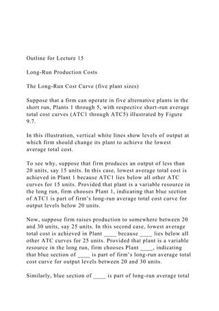
1. Outline for Lecture 15
Long-Run Production Costs
The Long-Run Cost Curve (five plant sizes)
Suppose that a firm can operate in five alternative plants in the
short run, Plants 1 through 5, with respective short-run average
total cost curves (ATC1 through ATC5) illustrated by Figure
9.7.
In this illustration, vertical white lines show levels of output at
which firm should change its plant to achieve the lowest
average total cost.
To see why, suppose that firm produces an output of less than
20 units, say 15 units. In this case, lowest average total cost is
achieved in Plant 1 because ATC1 lies below all other ATC
curves for 15 units. Provided that plant is a variable resource in
the long run, firm chooses Plant 1, indicating that blue section
of ATC1 is part of firm’s long-run average total cost curve for
output levels below 20 units.
Now, suppose firm raises production to somewhere between 20
and 30 units, say 25 units. In this second case, lowest average
total cost is achieved in Plant ____ because ____ lies below all
other ATC curves for 25 units. Provided that plant is a variable
resource in the long run, firm chooses Plant ____, indicating
that blue section of ____ is part of firm’s long-run average total
cost curve for output levels between 20 and 30 units.
Similarly, blue section of ____ is part of long-run average total

2. cost curve for output levels between 30 and 50 units, blue
section of ____ is part of long-run average total cost curve for
output levels between 50 and 60 units, and blue section of ____
is part of long-run average total cost curve for output levels
above 60 units.
Given these five cases illustrated by Figure 9.7, how do we
obtain long-run average total cost curve? Is it smooth or
bumpy? Explain.
The Long-Run Cost Curve (unlimited plant sizes)
The blue long-run average total cost curve in Figure 9.7 is
drawn under the assumption that firm can operate in five
alternative plants in the short run. However, in modern
manufacturing industries (i.e. automobiles, pharmaceuticals,
etc.) the number of possible plant sizes is many more than five.
In line with this reasoning, each red average total cost curve in
Figure 9.8 represents a possible plant size in the short run.
Given all these red curves illustrated by Figure 9.8, how do we
obtain long-run average total cost curve? Is it smooth or
bumpy? Explain.
Economies and Diseconomies of Scale
Shape of long-run average total cost curve (Figures 9.8 and 9.9)
is explained via economies and diseconomies of scale.
Economies of Scale
In the upper panel of Figure 9.9, economies of scale
corresponds to ____ part of the curve; in the output range
between zero and q1, average total cost ____ as production rises

3. in the long run.
Explain economies of scale: why is average total cost
decreasing with rising output?
Diseconomies of Scale
In the upper panel of Figure 9.9, diseconomies of scale explains
____ part of the curve; in the output range above than q2,
average total cost ____ as production rises in the long run.
Explain diseconomies of scale: why is average total cost
increasing with rising output?

4. Materials for Lecture 15
Start with textbook to get familiar with content and progression
of the lecture. Then, go to videos (and supplemental articles, if
provided) for further clarification and additional examples.
Textbook
Read carefully pages 209 through 213 from textbook.
Video
Comprehensive video on long-run average total cost curve,
economies of scale, and diseconomies of scale
http://www.youtube.com/watch?v=68-vmWJQqlo
Article
Article on cloud computing with a focus on economies of scale
http://www.cnet.com/news/james-hamilton-on-cloud-economies-
of-scale/
Outline for Lecture 16
Four Market Models

5. Pure Competition
What is the number of firms in a purely competitive market:
one, few, many, or a very large number? How would you
characterize products sold in a purely competitive market:
unique, differentiated, or standardized? Provide an example of a
purely competitive market.
Pure Monopoly
What is the number of firms in a purely monopolistic market:
one, few, many, or a very large number? How would you
characterize products sold in a purely monopolistic market:
unique, differentiated, or standardized?Provide an example of a
purely monopolistic market.
Monopolistic Competition
What is the number of firms in a monopolistically competitive
market: one, few, many, or a very large number? How would
you characterize products sold in a monopolistically
competitive market: unique, differentiated, or standardized?
Provide an example of a monopolistically competitive market.
Oligopoly
What is the number of firms in an oligopolistic market: one,
few, many, or a very large number? How would you
characterize products sold in an oligopolistic market: unique,
differentiated, or standardized? Provide an example of an
oligopolistic market.
Pure Competition: Characteristics and Occurrence
Purely competitive markets have four main characteristics.

6. 1. Very large numbers
Referring to your example of a purely competitive market from
above, how many firms would you expect to see in this market?
How would you characterize the extent of interdependence; do
one firm’s actions affect other firms? Explain.
2. Standardized product
Referring to your example from above, how similar are products
sold by different firms? Do consumers prefer one firm’s product
over another’s? Explain.
3. Price takers
Referring to your example from above, how much of total
output is produced by an individual competitive firm: all of it, a
large fraction, or a small fraction? Accordingly, would you
characterize individual firm as a price maker or a price taker?
Explain.
4. Free entry and exit
Referring to your example from above, how would you
characterize the ease with which firms can enter or exit
competitive industries? Explain.

7. Materials for Lecture 16
Start with textbook to get familiar with content and progression
of the lecture. Then, go to videos (and supplemental articles, if
provided) for further clarification and additional examples.
Textbook

8. Read carefully pages 221 and 222 from textbook.
Video
Four market models
http://www.youtube.com/watch?v=9Hxy-
TuX9fs&index=29&list=PL336C870BEAD3B58B
Perfect competition in first three minutes
http://www.youtube.com/watch?feature=fvwp&v=61GCogalzVc
&NR=1
Airline industry as an example of competitive markets (not a
great one) in first five minutes
https://www.khanacademy.org/economics-finance-
domain/microeconomics/perfect-competition-topic/perfect-
competition/v/perfect-competition
Outline for Lecture 17
Demand as Seen by a Purely Competitive Seller
Perfectly Elastic Demand
Figure 10.1 and accompanying table present price, quantity, and
revenue data for a purely competitive firm.
In the first two columns, we see that market price remains fixed
at ____ as quantity demanded increases from 0 to 10 units.
Explain why.
As a result, competitive firm’s demand curve will plot as a ____
at the level of market price.

9. Average, Total, and Marginal Revenue
Total Revenue
How do we define total revenue?
According to Table 10.1, what is total revenue from selling one
unit of output? How about two units? Report the total revenue
for all remaining output levels.
Based on these data, how do we graphically illustrate total
revenue?
Average Revenue
How do we define average revenue?
In Table 10.1, what is average revenue from selling one unit of
output? How about two units? Report the average revenue for
all remaining output levels.
Based on these data, how do we graphically illustrate average
revenue? Does average revenue curve coincide with demand
curve? Explain.
Marginal Revenue
How do we define marginal revenue?
In Table 10.1, what is marginal revenue from first unit of
output? How about second unit? Report the marginal revenue
for all remaining output levels.
Based on these data, how do we graphically illustrate marginal
revenue? Does marginal revenue curve coincide with demand

10. and average revenue curves? Explain.
Profit Maximization in the Short Run: Marginal Revenue-
Marginal Cost Approach
Profit maximization by a competitive firm in the short run rests
on two cases regarding marginal revenue and marginal cost.
Case 1
Assuming that producing is preferable to shutting down in the
short run, competitive firm should produce any unit of output
whose ____ exceeds ____. Explain why.
Case 2
Assuming that producing is preferable to shutting down in the
short run, competitive firm should not produce an output level if
____ exceeds ____. Explain why.
Rule
Combining these two cases, we obtain the following rule
As long as producing is preferable to shutting down,
competitive firm maximizes profits in the short run by
producing the level of output at which marginal revenue ____
marginal cost.

11. Materials for Lecture 17
Start with textbook to get familiar with content and progression
of the lecture. Then, go to videos (and supplemental articles, if
provided) for further clarification and additional examples.
Textbook
Read carefully pages 222 through 226 from textbook.
Video
Competitive markets, determination of market price via industry
demand and industry supply, and output determination by
competitive firm in first five minutes
https://www.youtube.com/watch?v=61GCogalzVc&list=PL336C
870BEAD3B58B&index=29

12. Graphical analysis of profit maximization
https://www.youtube.com/watch?v=J_tdZZkRvbg&list=PL336C
870BEAD3B58B&index=30
Comprehensive video on competitive markets answering
questions from Lectures 16 and 17
http://www.youtube.com/watch?v=ivBLIlhag5w
Outline for Lecture 18
Depending on market price (determined by market demand and
market supply), competitive firm faces three scenarios in the
short run: profit maximization, loss minimization, and
shutdown.
Profit-Maximizing Case
First five columns of the table accompanying Figure 10.3
present cost data for a competitive firm. In the 6th column, we
have the market price of ____, which also equals marginal
revenue.
Applying MR = MC rule, how many units of output will
competitive firm produce to maximize profits in the short run?
Explain.
Total profit equals per-unit profit multiplied by quantity sold.
What is per-unit profit in this case? What is quantity sold?
Given these two figures, what is total profit?
Figure 10.3 illustrates profit-maximizing case: average variable
cost (AVC) curve and average total cost (ATC) curve are U-
shaped; marginal cost (MC) curve is also U-shaped and it

13. intersects AVC and ATC at their ____; MR = Price line is
drawn at the market price of ____.
In applying MR = MC rule, we look for the intersection of ____
with ____, which yields an output of ____ units. At this output
level, market price (P) of ____ exceeds average total cost (A) of
____, thereby producing a per-unit profit of ____. Per-unit
profit is multiplied by output produced to give a total profit of
____, which is illustrated by the area of ____.
Loss-Minimizing Case
If market price falls to $81, competitive firm will face loss
minimization.
First five columns of the table accompanying Figure 10.4
present cost data. In the 6th column, we have the new, lower
market price of ____, which also equals marginal revenue.
Applying MR = MC rule, how many units of output will
competitive firm produce to minimize losses in the short run?
Explain.
Total loss equals per-unit loss multiplied by quantity sold. What
is per-unit loss in this case? What is quantity sold? Given these
two figures, what is total loss?
Figure 10.4 illustrates loss-minimizing case. It is identical to
Figure 10.3, except MR = Price line is drawn at the new, lower
market price of ____.
In applying MR = MC rule, we look for the intersection of ____
with ____, which yields an output of ____ units. At this output
level, average total cost (A) of ____ exceeds market price (P) of
____, thereby producing a per-unit loss of ____. Per-unit loss is
multiplied by output produced to give a total loss of ____,

14. which is illustrated by the area of ____.
Shutdown Case
If market price falls further to $71, competitive firm will shut
down in the short run.
First five columns of the table accompanying Figure 10.4
present cost data. In the 8th column, we have the new, lowest
market price of ____, which also equals marginal revenue.
In the 9th column, what is total loss at an output of zero? How
about an output of one? Report the total loss for remaining
output levels. Based on these figures, what is the best short-run
decision for competitive firm: keep producing or shut down?
Explain.

15. Materials for Lecture 18
Start with textbook to get familiar with content and progression
of the lecture. Then, go to videos (and supplemental articles, if
provided) for further clarification and additional examples.
Textbook
Read carefully pages 226 through 230 from textbook.
Video
Profit-maximizing case after three minute mark
https://www.youtube.com/watch?v=61GCogalzVc&list=PL336C
870BEAD3B58B&index=29
How falling market price leads to loss-minimizing and
shutdown cases
http://www.youtube.com/watch?v=_-OWuxR0-V8

16. 1