SlideShare a Scribd company logo
1 of 59
R. GLENN
HUBBARD
Economics
FOURTH EDITION
ANTHONY PATRICK
O’BRIEN
1
Chapter Outline and
Learning Objectives15.1Is Any Firm Ever Really a
Monopoly?15.2Where Do Monopolies Come From?15.3How
Does a Monopoly Choose Price and Output?15.4Does Monopoly
Reduce Economic Efficiency?15.5Government Policy toward
Monopoly
Monopoly and
Antitrust Policy
CHAPTER
15
‹#› of 42
© 2013 Pearson Education, Inc. Publishing as Prentice Hall
Monopoly is a market structure consisting of a firm that is the
only seller of a good or service that does not have a close
substitute.
Monopoly exists at the opposite end of the competition
spectrum to perfect competition.
We study monopolies for two reasons:
Some firms truly are monopolists, so it is important to
understand how they behave.
Firms might collude in order to act like a monopolist, with
important implications for firm behavior.
What is a monopoly, and why do we study them?
‹#› of 42
© 2013 Pearson Education, Inc. Publishing as Prentice Hall
3
Define monopoly.
15.1 LEARNING OBJECTIVE
Is Any Firm Ever Really a Monopoly?
‹#› of 42
© 2013 Pearson Education, Inc. Publishing as Prentice Hall
4
It is reasonable to ask whether monopolies truly ever exist.
For example, suppose you live in a small town with only one
pizzeria. Is that pizzeria a monopoly?
It has competition from other fast-food restaurants
It has competition from grocery stores that provide pizzas for
you to cook at home
If you consider these alternatives to be close substitutes for
pizzeria pizza, then the pizza restaurant is not a monopoly.
If you do not consider these alternatives to be close substitutes
for pizzeria pizza, then the pizza restaurant is a monopoly.
Regardless, the pizzeria’s unique position may afford it some
monopoly power to raise prices, and obtain positive economic
profit.
Are there really monopolies?
‹#› of 42
© 2013 Pearson Education, Inc. Publishing as Prentice Hall
5
Is Google a Monopoly?
Making
the
Connection
Although there are many other firms that offer search engines,
Google has a dominant market share: 70% in the U.S., and 90%
in Europe.
In the strictest sense, Google is not a monopoly in the search-
engine market. But its dominant market position provides it
with many advantages, like the ability to exclude competitors
from its content.
Of course, Google argues that its superiority is what has caused
the high market share.
Modern governments realize that monopolies are generally “bad
for consumers”, and discourage their existence.
‹#› of 42
© 2013 Pearson Education, Inc. Publishing as Prentice Hall
6
Explain the four main reasons monopolies arise.
15.2 LEARNING OBJECTIVE
Where Do Monopolies Come From?
‹#› of 42
© 2013 Pearson Education, Inc. Publishing as Prentice Hall
7
For a firm to exist as a monopoly, there must be barriers to
entry preventing other firms coming in and competing with it.
The four main reasons for these barriers to entry are:
Government restrictions on entry
Exclusive control over a key resource
Network externalities
Natural monopoly
The next few slides will examine these in detail.
Reasons for monopoly existence
‹#› of 42
© 2013 Pearson Education, Inc. Publishing as Prentice Hall
8
In the U.S., governments block entry in two main ways:
Patents and copyrights
Newly developed products like drugs are frequently granted
patents, the exclusive right to produce a product for a period of
20 years from the date the patent is filed with the government.
Similarly, copyrights provide the exclusive right to produce and
sell creative works like books and films.
Patents and copyrights encourage innovation and creativity,
since without them, firms would not be able to substantially
profit from their endeavors.
Public franchises
A government designation that a firm is the only legal provider
of a good or service is known as a public franchise. These might
exist, for example, in electricity or water markets.
1. Government restrictions on entry
‹#› of 42
© 2013 Pearson Education, Inc. Publishing as Prentice Hall
9
For many years, the Aluminum Company of America (Alcoa)
either owned or had long-term contracts for almost all the
world’s supply of bauxite, the mineral from which we obtain
aluminum.
Such control over a key resource served as a substantial barrier
to entry for additional firms.
The National Football League (NFL) acts as a monopoly in this
manner too: it ensures that the majority of the world’s best
football players are under contract to the NFL, and unable to be
used for another potential league.
2. Exclusive control over a key resource
‹#› of 42
© 2013 Pearson Education, Inc. Publishing as Prentice Hall
10
The End of the Christmas Plant Monopoly
Making
the
Connection
For many years, the Paul Ecke Ranch in Encinitas, CA, had a
monopoly on poinsettias.
Ecke had exclusive control over a key resource: a botanical
secret he discovered that allowed multiple branches to grow
from one stem of the native Mexican wildflower.
Eventually, a researcher discovered Ecke’s secret, and
published it.
The result: the barriers to entry were broken, and competitors
quickly mimicked Ecke’s poinsettias. Prices fell quickly to the
competitive level, eroding Ecke’s economic profits.
‹#› of 42
© 2013 Pearson Education, Inc. Publishing as Prentice Hall
11
Are Diamond Profits Forever?
The De Beers Diamond Monopoly
Making
the
Connection
The most famous monopoly based on control of a raw material
is the De Beers diamond monopoly.
The South African De Beers firm sought to control as much of
the supply of diamonds as possible, resulting in it being able to
keep prices high.
By 2000, new competitors had eroded De Beers’ control of the
world’s diamond production to 40%
Seeking to maintain its monopoly power, De Beers has started
branding its diamonds with a “Forevermark”, supposedly
indicating high quality. Do you think this marketing strategy
will be successful long-term?
‹#› of 42
© 2013 Pearson Education, Inc. Publishing as Prentice Hall
12
Economists refer to network externalities as a situation in which
the usefulness of a product increases with the number of
consumers who use it.
Examples: HD televisions
Computer operating systems (like Windows)
Social networking sites (like Facebook)
These network externalities can set off a virtuous cycle for a
firm, allowing the value of its product to continue to increase,
along with the price it can charge.
But consumers may be locked into an inferior product.
3. Network externalities
‹#› of 42
© 2013 Pearson Education, Inc. Publishing as Prentice Hall
13
A natural monopoly occurs when economies of scale are so
large that one firm can supply the entire market at a lower
average total cost than can two or more firms.
4. Natural monopoly
Figure 15.1
In the market for electricity delivery, a single firm (point A)
can deliver electricity at a lower cost than can two firms (point
B).
This is often because of high fixed costs; in this example, the
cost of erecting power lines and transformers, for example.
‹#› of 42
© 2013 Pearson Education, Inc. Publishing as Prentice Hall
14
Explain how a monopoly chooses price and output.
15.3 LEARNING OBJECTIVE
How Does a Monopoly Choose Price and Output?
‹#› of 42
© 2013 Pearson Education, Inc. Publishing as Prentice Hall
15
In our study of oligopoly, we abandoned the idea of marginal
cost and marginal revenue, because the strategic interaction
between firms overrode these concepts.
Monopolists have no competitors, and hence no concern about
strategic interactions.
They seek to maximize profit by choosing a quantity to produce,
just like perfect and monopolistic competitors.
In fact, monopolists act very much like monopolistic
competitors: they face a downward sloping demand curve.
The difference is that barriers to entry will prevent other firms
from competing away their economic profit.
The return of marginal cost and marginal revenue
‹#› of 42
© 2013 Pearson Education, Inc. Publishing as Prentice Hall
16
Time Warner Cable is a monopolist in the market for cable
television services.
The first two columns of the table show the market demand
curve, which is also Time Warner’s demand curve.
Total, average, and marginal revenue are all calculated in the
usual manner.
Calculating a monopoly’s revenue
‹#› of 42
© 2013 Pearson Education, Inc. Publishing as Prentice Hall
17
Figure 15.2
As the monopolist seeks to expand its output, two effects occur:
Revenue increases from selling an additional unit of output at
whatever price is necessary to convince an additional customer
to purchase it.
Revenue decreases, because the price reduction is shared with
existing customers.
Graphing a monopoly’s revenue
So marginal revenue is always below demand for a monopolist.
‹#› of 42
© 2013 Pearson Education, Inc. Publishing as Prentice Hall
18
Figure 15.3
The monopolist maximizes profit by producing the quantity
where the additional revenue from the last unit (marginal
revenue) just equals the additional cost incurred from its
production (marginal cost).
MC = MR determines quantity for a monopolist.
Profit-maximizing price and output for a monopoly
‹#› of 42
© 2013 Pearson Education, Inc. Publishing as Prentice Hall
19
Figure 15.3
At this quantity,
The demand curve determines price, and
The average total cost (ATC) curve determines average cost.
Profit is the difference between these (P–ATC), times quantity
(Q).
Profit-maximizing price and output for a monopoly
‹#› of 42
© 2013 Pearson Education, Inc. Publishing as Prentice Hall
20
Since there are barriers to entry, additional firms cannot enter
the market.
So there is no distinction between the short run and long run for
a monopoly.
Then unlike for monopolistic competition, we expect
monopolists to continue to earn profits in the long run.
Long-run profits
‹#› of 42
© 2013 Pearson Education, Inc. Publishing as Prentice Hall
21
Use a graph to illustrate how a monopoly affects economic
efficiency.
15.4 LEARNING OBJECTIVE
Does Monopoly Reduce Economic Efficiency?
‹#› of 42
© 2013 Pearson Education, Inc. Publishing as Prentice Hall
Suppose that a market could be characterized by either perfect
competition or monopoly. Which would be better?
The thought experiment here is to suppose there is some market
that is perfectly competitive, say the wholesale market for
potatoes.
Then a single firm buys up all of the potato farms in the
country.
What would happen to:
Price of potatoes?
Quantity of potatoes traded?
The net benefit of consumers (i.e. consumer surplus)?
The net benefit of producers (i.e. producer surplus)?
The net benefit of all of society (i.e. economic surplus)?
Comparing perfect competition and monopoly
‹#› of 42
© 2013 Pearson Education, Inc. Publishing as Prentice Hall
23
Figure 15.4
The market for potatoes is initially perfectly competitive.
Price is PC, quantity traded is QC.
Now the market is supplied by a single firm. Since the single
firm is made up of all of the smaller firms, the marginal cost
curve for this new firm is identical to the old supply curve.
If a perfect competition becomes a monopoly…
‹#› of 42
© 2013 Pearson Education, Inc. Publishing as Prentice Hall
24
Figure 15.4
But the new firm maximizes market profit, producing the
quantity where marginal cost equals marginal revenue (MC =
MR).
This quantity (QM) is lower than the competitive quantity (QC).
The firm charges the corresponding price on the demand curve,
PM. This price is higher than the competitive price, PC.
… quantity will fall and price will rise
‹#› of 42
© 2013 Pearson Education, Inc. Publishing as Prentice Hall
25
Fewer potatoes will be traded at a higher price.
Consumer surplus will fall (with the higher price).
Producer surplus must rise, otherwise the firm would have
chosen the perfectly competitive price and quantity.
Could the increase in producer surplus offset the decrease in
consumer surplus?
No! Perfectly competitive markets maximized the economic
(total) surplus in a market; if fewer trades take place, the
economic surplus must fall.
Measuring the efficiency loss from monopoly
‹#› of 42
© 2013 Pearson Education, Inc. Publishing as Prentice Hall
26
With the higher monopoly price, consumer surplus decreases by
the areas A+B.
Producer surplus falls by C, but rises by A; an overall increase.
Area A simply is simply a transfer of surplus: neither inherently
good nor bad.
But areas B and C are lost surpluses: deadweight loss.
Figure 15.5
The inefficiency of monopoly
‹#› of 42
© 2013 Pearson Education, Inc. Publishing as Prentice Hall
Recall that a market has productive efficiency if output is
produced as cheaply as possible.
That is still the case here: the QM units of output are produced
at their lowest possible cost.
But we lose allocative efficiency: the cost to society of the last
unit produced (MCM) is not the same as the benefit to society
of the last unit (PM).
Figure 15.5
Productive or allocative inefficiency?
‹#› of 42
© 2013 Pearson Education, Inc. Publishing as Prentice Hall
There are relatively few monopolies, so the loss of economic
efficiency due to monopolies must be relatively small.
But many firms have market power: the ability of a firm to
charge a price greater than marginal cost.
In fact, the only firms that do not have market power are
perfectly competitive firms; and perfect competition is rare.
Economists estimate that overall, the loss of efficiency in the
United States due to market power is probably less than 1% of
total U.S. production—about $480 per person annually.
Why so low? Most firms face a relatively large degree of
competition, resulting in prices much closer to marginal cost
than we would see with monopolies.
So deadweight loss due to market power is relatively small.
How large are these efficiency losses?
‹#› of 42
© 2013 Pearson Education, Inc. Publishing as Prentice Hall
29
Market power may produce some benefit for an economy: the
prospect of market power (and the resulting economic profits)
drives firms to innovate, creating new products and services.
This drive affects large firms—who reinvest profits in the hope
of making larger future profits—and small firms—who hope to
obtain profits for themselves—alike.
The Austrian economist Joseph Schumpeter claimed that this
drive would create a “gale of creative destruction” that would
eventually benefit consumers more than increased price
competition.
This helps to explain governmental ambivalence regarding large
firms with market power.
An argument in favor of market power
‹#› of 42
© 2013 Pearson Education, Inc. Publishing as Prentice Hall
30
Discuss government policies toward monopoly.
15.5 LEARNING OBJECTIVE
Government Policy toward Monopoly
‹#› of 42
© 2013 Pearson Education, Inc. Publishing as Prentice Hall
In the 1870s and 1880s, several “trusts” had formed: boards of
trustees that oversaw the operation of several firms in an
industry, and enforced collusive agreements.
This helped prompt U.S. antitrust laws, aimed at eliminating
collusion and promoting competition among firms. The most
important of these laws are detailed below.
Antitrust laws and antitrust enforcement
Table 15.1LawDate Enacted PurposeSherman
Act1890Prohibited “restraint of trade,” including price fixing
and collusion. Also outlawed monopolization.Clayton
Act1914Prohibited firms from buying stock in competitors and
from having directors serve on the boards of competing
firms.Federal Trade Commission Act1914Established the
Federal Trade Commission (FTC) to help administer antitrust
laws.Robinson-Patman Act1936Prohibited firms from charging
buyers different prices if the result would reduce
competition.Cellar-Kefauver Act1950Toughened restrictions on
mergers by prohibiting any mergers that would reduce
competition.
‹#› of 42
© 2013 Pearson Education, Inc. Publishing as Prentice Hall
32
The Federal government is particularly concerned about
horizontal mergers: mergers between firms in the same industry,
as opposed to vertical mergers between two firms at different
stages of the production process.
Such mergers are likely enhance firms’ market power.
The graph shows such a merger, increasing the price from the
competitive price (PC) to the monopoly price (PM), and
resulting in deadweight loss.
Mergers without efficiency gains
Figure 15.6
‹#› of 42
© 2013 Pearson Education, Inc. Publishing as Prentice Hall
33
Firms seeking to merge typically argue that the resulting larger
firm will have lower costs, and hence be able to produce more
efficiently.
Then even if they charge the (new) monopoly price, the result is
an improvement for consumers.
However, costs may not decrease by as much as the firms claim,
resulting in consumers being worse off.
Economists with the FTC and Department of Justice review
potential mergers one-by-one.
Mergers with efficiency gains
Figure 15.6
‹#› of 42
© 2013 Pearson Education, Inc. Publishing as Prentice Hall
34
Economists and lawyers at the Department of Justice and the
Federal Trade Commission developed guidelines for themselves
and firms to use in evaluating whether potential merger was
acceptable.
These include:
Market definition
Measure of concentration
Merger standards
DOJ and FTC merger guidelines
‹#› of 42
© 2013 Pearson Education, Inc. Publishing as Prentice Hall
35
Suppose Hershey Foods sought to merge with Mars Inc.
In what market do these firms compete? The market for candy?
The market for snacks? The market for all food?
The more broadly defined the market, the smaller (and more
harmless) the merger appears.
To determine the appropriate scope of the market, the
government tries to determine which goods are close substitutes
for those produced by the firms.
The “appropriate market” is defined as the smallest market
containing the firms’ products for which an overall price rise
within the market would result in total market profits
increasing.
(If profits would decrease, there must be adequate substitutes
available; hence the market is too narrowly defined.)
1. Market definition
‹#› of 42
© 2013 Pearson Education, Inc. Publishing as Prentice Hall
36
Four-firm concentration ratios (the percentage of industry sales
accounted for by the four largest firms) can be useful, but the
government seeks a more detailed overall picture of the
industry.
For this, it uses the Herfindahl-Hirschman Index (HHI), created
by squaring the percentage market shares of each firm, and
adding up the results.
Some examples are given below:
2. Measure of concentrationFirm market
sharesFormulaHHI100%100210,00050%, 50%502 +
5025,00030%, 30%, 20%, 20%302 + 302 + 202 +
2022,60010%, 10%, …, 10%10 x 1021,000
‹#› of 42
© 2013 Pearson Education, Inc. Publishing as Prentice Hall
37
Based on the calculated HHI values, the DOJ and FTC apply the
following standards to determine if they ought to challenge the
potential merger of two or more firms:
Firms having their merger applications challenged must satisfy
the DOJ and FTC that their merger would result in substantial
efficiency gains. The burden of proof is on the merging firms.
3. Merger standardsIncrease in HHIPost-merger HHI< 100100 –
200> 200< 1,500Challenge unlikelyChallenge
unlikelyChallenge unlikely1,500 – 2,500Challenge
unlikelyChallenge possibleChallenge possible> 2,500Challenge
unlikelyChallenge possibleChallenge very likely
‹#› of 42
© 2013 Pearson Education, Inc. Publishing as Prentice Hall
http://www.ftc.gov/os/2010/08/100819hmg.pdf ; see page 19
38
Should AT&T Have Been Allowed to Merge
with T-Mobile?
Making
the
Connection
In early 2011, AT&T agreed to buy T-Mobile. As the second-
and fourth-largest mobile wireless providers in the U.S., this
merger would have created a large increase in market
concentration: increasing the HHI by over 700 points.
The firms claimed that they could operate more efficiently
together: closing hundreds of redundant retail stores, and
combining their technical and support staff. AT&T estimated
cost savings of $3 billion per year.
After several months of study, the DOJ filed suit to block the
merger, rejecting AT&T’s cost savings estimate. In late 2011,
AT&T admitted defeat, and dropped its merger plans.
‹#› of 42
© 2013 Pearson Education, Inc. Publishing as Prentice Hall
Natural monopolies have the potential to serve customers more
cheaply than multiple firms. But the usual market forces that
drive price down do not exist.
Local and/or state regulatory commissions typically set prices
for these natural monopolies, instead of allowing the firms to
set their own price.
But that raises the question: what price should the regulators
choose?
A price that makes the monopoly make zero profit?
The efficient price that would maximize consumer welfare?
Regulating natural monopolies
‹#› of 42
© 2013 Pearson Education, Inc. Publishing as Prentice Hall
40
Figure 15.7
If the natural monopoly were not subject to regulation, it would
choose quantity QM and price PM.
Efficiency (MC = MR) suggests a price of QE. But then the firm
makes a loss.
Regulating natural monopolies
The typical compromise is to allow the firm to charge a price
where it can make zero economic profit: PR. The resulting
quantity QR is hopefully close to the efficient level, keeping
deadweight loss small.
‹#› of 42
© 2013 Pearson Education, Inc. Publishing as Prentice Hall
41
Monopoly is a market structure; natural monopoly is a reason
the monopoly market structure might exist. Monopolies need
not be natural monopolies.
No monopolist, not even a natural monopolist, tries to minimize
cost. MC = MR guides an (unregulated) monopolist.
While our graphs tend to show the efficiency loss from
monopolies to be high, estimates of the efficiency loss due to
all market power are really quite low: <1% of total output.
Common misconceptions to avoid
‹#› of 42
© 2013 Pearson Education, Inc. Publishing as Prentice Hall
42
R. GLENN
HUBBARD
Economics
FOURTH EDITION
ANTHONY PATRICK
O’BRIEN
1
Firms in Perfectly Competitive Markets
CHAPTER
12
Chapter Outline and
Learning Objectives12.1Perfectly Competitive
Markets12.2How a Firm Maximizes Profit in a Perfectly
Competitive Market12.3Illustrating Profit or Loss on the Cost
Curve Graph12.4Deciding Whether to Produce or to Shut Down
in the Short Run12.5“If Everyone Can Do It, You Can’t Make
Money at It”: The Entry and Exit of Firms in the Long
Run12.6Perfect Competition and Efficiency
‹#› of 46
© 2013 Pearson Education, Inc. Publishing as Prentice Hall
For the next few chapters, we will examine several different
market structures: models of how the firms in a market interact
with buyers to sell their output.
The market structures we will examine are, in decreasing order
of competitiveness:
Perfectly competitive markets
Monopolistically competitive markets
Oligopolies, and
Monopolies.
Each market structure will be applicable to different real-world
markets, and will give us insight into how firms in certain types
of markets behave.
Market structures
‹#› of 46
© 2013 Pearson Education, Inc. Publishing as Prentice Hall
3
Table 12.1Market StructureCharacteristicPerfect
CompetitionMonopolistic
CompetitionOligopolyMonopolyNumber of
firmsManyManyFewOneType of
productIdenticalDifferentiatedIdentical or
differentiatedUniqueEase of entryHighHighLowEntry
blockedExamples of industries• Growing wheat
• Growing apples• Clothing stores
• Restaurants• Manufacturing computers
• Manufacturing automobiles• First-class mail delivery
• Tap water
The following table identifies the characteristics that determine
the type of market.
Table of market structures
‹#› of 46
© 2013 Pearson Education, Inc. Publishing as Prentice Hall
4
Explain what a perfectly competitive market is and why a
perfect competitor faces a horizontal demand curve.
12.1 LEARNING OBJECTIVE
Perfectly Competitive Markets
‹#› of 46
© 2013 Pearson Education, Inc. Publishing as Prentice Hall
The first market structure we will examine is the perfectly
competitive market: one in which
There are many buyers and sellers;
All firms sell identical products; and
There are no barriers to new firms entering the market
The first and second conditions imply that perfectly competitive
firms are price-takers: they are unable to affect the market
price. This is because they are tiny relative to the market, and
sell exactly the same product as everyone else.
As you might have already guessed, perfectly competitive
markets are relatively rare.
Introduction to perfectly competitive markets
‹#› of 46
© 2013 Pearson Education, Inc. Publishing as Prentice Hall
Figure 12.1
By definition, a perfectly competitive firm is too small to affect
the market price.
Agricultural markets, like the market for wheat, are often
thought to be close to perfectly competitive.
Suppose you are a wheat farmer; whether you sell 6,000…
… or 15,000 bushels of wheat, you receive the same price per
bushel: you are too small to affect the market price.
The demand curve for a perfectly competitive firm
‹#› of 46
© 2013 Pearson Education, Inc. Publishing as Prentice Hall
7
There are thousands of individual wheat farmers.
Their collective supply, combined with the overall market
demand for wheat, determines the market price of wheat.
The individual farmer takes this market price as his or her
demand curve.
How is the firm’s demand curve determined?
Figure 12.2
‹#› of 46
© 2013 Pearson Education, Inc. Publishing as Prentice Hall
8
Explain how a firm maximizes profit in a perfectly competitive
market.
12.2 LEARNING OBJECTIVE
How a Firm Maximizes Profit in a Perfectly Competitive Market
‹#› of 46
© 2013 Pearson Education, Inc. Publishing as Prentice Hall
We assume that all firms try to maximize profits—including
perfectly competitive ones.
Recall that
Profit = Total Revenue – Total Cost
Revenue for a perfectly competitive firm is easy to analyze: the
firm receives the same amount of money for every unit of
output it sells. So
Price = Average Revenue = Marginal Revenue
This is illustrated in the table on the next slide.
Profit maximization as the goal of the firm
‹#› of 46
© 2013 Pearson Education, Inc. Publishing as Prentice Hall
Number of Bushels
(Q)Market Price
(per bushel)
(P)Total
Revenue
(TR)Average Revenue
(AR)Marginal Revenue
(MR)0
1
2
3
4
5
6
7
8
9
10$4
4
4
4
4
4
4
4
4
4
4$0
4
8
12
16
20
24
28
32
36
40—
$4
4
4
4
4
4
4
4
4
4—
$4
4
4
4
4
4
4
4
4
4
Table 12.2
For a firm in a perfectly competitive market, price is equal to
both average revenue and marginal revenue.
Revenues for a perfectly competitive firm
‹#› of 46
© 2013 Pearson Education, Inc. Publishing as Prentice Hall
11
Quantity
(bushels)
(Q)Total
Revenue
(TR)Total
Cost
(TC)
Profit
(TR−TC)Marginal Revenue
(MR)Marginal Cost
(MC)0
1
2
3
4
5
6
7
8
9
10$0.00
4.00
8.00
12.00
16.00
20.00
24.00
28.00
32.00
36.00
40.00$2.00
5.00
7.00
8.50
10.50
13.00
16.50
21.50
28.50
38.00
50.50−$2.00
−1.00
1.00
3.50
5.50
7.00
7.50
6.50
3.50
−2.00
−10.50—
$4.00
4.00
4.00
4.00
4.00
4.00
4.00
4.00
4.00
4.00—
$3.00
2.00
1.50
2.00
2.50
3.50
5.00
7.00
9.50
12.50
Table 12.3
Profit maximization as the goal of the firm
Suppose costs are as in the table.
We can calculate profit; profit is maximized at a quantity of 6
bushels. This is the profit-maximizing level of output.
‹#› of 46
© 2013 Pearson Education, Inc. Publishing as Prentice Hall
12
Quantity
(bushels)
(Q)Total
Revenue
(TR)Total
Cost
(TC)
Profit
(TR−TC)Marginal Revenue
(MR)Marginal Cost
(MC)0
1
2
3
4
5
6
7
8
9
10$0.00
4.00
8.00
12.00
16.00
20.00
24.00
28.00
32.00
36.00
40.00$2.00
5.00
7.00
8.50
10.50
13.00
16.50
21.50
28.50
38.00
50.50−$2.00
−1.00
1.00
3.50
5.50
7.00
7.50
6.50
3.50
−2.00
−10.50—
$4.00
4.00
4.00
4.00
4.00
4.00
4.00
4.00
4.00
4.00—
$3.00
2.00
1.50
2.00
2.50
3.50
5.00
7.00
9.50
12.50
Table 12.3
Profit maximization as the goal of the firm
We can also calculate marginal revenue and marginal cost for
the firm.
Profit is maximized by producing as long as MR>MC; or until
MR=MC, if that is possible.
‹#› of 46
© 2013 Pearson Education, Inc. Publishing as Prentice Hall
13
Figure 12.3a
If we show total revenue and total cost on the same graph, the
vertical difference between the two curves is the profit the firm
makes.
(Or the loss, if costs are greater than revenues.)
At the profit-maximizing level of output, this (positive) vertical
distance is maximized.
Showing revenue, cost, and profit
‹#› of 46
© 2013 Pearson Education, Inc. Publishing as Prentice Hall
14
It is generally easier to determine the profit-maximizing level of
output on a graph of marginal revenue and marginal cost.
Marginal revenue is constant and equal to price for the perfectly
competitive firm.
The firm maximizes profit by choosing the level of output
where marginal revenue is equal to marginal cost (or just less, if
equal is not possible).
Figure 12.3b
Showing marginal revenue and marginal cost
‹#› of 46
© 2013 Pearson Education, Inc. Publishing as Prentice Hall
15
The rules we have just developed for profit maximization are:
The profit-maximizing level of output is where the difference
between total revenue and total cost is greatest; and
The profit-maximizing level of output is also where MR = MC.
However neither of these rules require the assumption of perfect
competition; they are true for every firm!
For perfectly competitive firms, we can develop an additional
rule, because for those firms, P = MR; this implies:
The profit-maximizing level of output is also where P = MC.
Rules for profit maximization
‹#› of 46
© 2013 Pearson Education, Inc. Publishing as Prentice Hall
Use graphs to show a firm’s profit or loss.
12.3 LEARNING OBJECTIVE
Illustrating Profit or Loss on the Cost Curve Graph
‹#› of 46
© 2013 Pearson Education, Inc. Publishing as Prentice Hall
We know profit equals total revenue minus total cost; and total
revenue is price times quantity. So write:
Dividing both sides by Q, we obtain:
The “Q”s cancel in the first term, and the second is average
total cost; so we can write:
Multiplying both sides by Q, we obtain:
The right hand side is the area of a rectangle with height (P –
ATC) and length Q. We can use this to illustrate profit on a
graph.
A useful formula for profit
‹#› of 46
© 2013 Pearson Education, Inc. Publishing as Prentice Hall
Figure 12.4
A firm maximizes profit at the level of output at which marginal
revenue equals marginal cost.
The difference between price and average total cost equals
profit per unit of output.
Showing a profit on the graph
Total profit equals profit per unit of output, times the amount of
output: the area of the green rectangle on the graph.
‹#› of 46
© 2013 Pearson Education, Inc. Publishing as Prentice Hall
19
Figure 12.4
It is a very common error to believe the firm should produce at
Q1: the level of output where profit per unit is maximized.
But this does NOT maximize overall profit; the next few units
of output bring in more marginal revenue than their marginal
cost.
Incorrect level of output
You can know this because MR>MC at Q1; this demonstrates
that Q1 is NOT the profit-maximizing level of output.
‹#› of 46
© 2013 Pearson Education, Inc. Publishing as Prentice Hall
20
We know we should produce at the level of output where
marginal cost equals marginal revenue (MC=MR).
We have been calling this the profit-maximizing level of output.
But what if the firm doesn’t make a profit at this level of
output, or at any other?
In this case, we would want to make the smallest loss possible.
Note that sometimes a loss may be unavoidable, if we have high
fixed costs.
It turns out that MC=MR is still the correct rule to use; it will
guide us to the loss-minimizing level of output.
Reinterpreting marginal cost equals marginal revenue
‹#› of 46
© 2013 Pearson Education, Inc. Publishing as Prentice Hall
Figure 12.5a
In the graph on the left, price never exceeds average cost, so the
firm could not possibly make a profit.
The best this firm can do is to break even, obtaining no profit
but incurring no loss.
The MC=MR rule leads us to this optimal level of production.
A firm breaking even
‹#› of 46
© 2013 Pearson Education, Inc. Publishing as Prentice Hall
22
Figure 12.5b
The situation is even worse for this firm; not only can it not
make a profit, price is always lower than average total cost, so
it must make a loss.
It makes the smallest loss possible by again following the
MC=MR rule.
No other level of output allows the firm’s loss to be so small.
A firm making a loss
‹#› of 46
© 2013 Pearson Education, Inc. Publishing as Prentice Hall
23
Once we have determined the quantity where MC=MR, we can
immediately know whether the firm is making a profit,
breaking even, or making a loss. At that quantity,
If P > ATC, the firm is making a profit
If P = ATC, the firm is breaking even
If P < ATC, the firm is making a loss
In fact, these statements hold true at every level of output.
Identifying whether or not a firm can make a profit
‹#› of 46
© 2013 Pearson Education, Inc. Publishing as Prentice Hall
24
Explain why firms may shut down temporarily.
12.4 LEARNING OBJECTIVE
Deciding Whether to Produce or to Shut Down in the Short Run
‹#› of 46
© 2013 Pearson Education, Inc. Publishing as Prentice Hall
Suppose a firm in a perfectly competitive market is making a
loss. It would like the price to be higher, but it is a price-taker,
so it cannot raise the price. That leaves two options:
Continue to produce, or
Stop production by shutting down temporarily
If the firm shuts down, it will still need to pay its fixed costs.
The firm needs to decide whether to incur only its fixed costs,
or to produce and incur some variable costs, but obtain some
revenue.
The firm’s fixed costs should be treated as sunk costs, costs that
have already been paid and cannot be recovered, because even if
they haven’t literally been paid yet, the firm is still obliged to
pay them.
Sunk costs should be irrelevant to your decision-making.
Responses of perfect competitors to losses
‹#› of 46
© 2013 Pearson Education, Inc. Publishing as Prentice Hall
26
Losing money on Chevy Volts
Making
the
Connection
In 2012, Chevrolet was facing intense criticism over its
production of the Volt, its small electric/gas hybrid car.
Critics pointed out that while Chevrolet sold the Volts for
around $40,000, the average total cost of a Volt was around
$80,000.
But this ATC included large (sunk) fixed costs for research and
development; Chevy actually increased profit (decreased loss)
by around $15,000 on each additional Volt it sold.
Stopping production and sales would have resulted in a larger
loss on the Volt than what Chevy actually achieved.
Whether it should have initially invested in the hybrid vehicle
research that led to the Volt is debatable; but once it had done
so, Chevy would have been foolish to stop production just
because sales were weaker than they had hoped.
‹#› of 46
© 2013 Pearson Education, Inc. Publishing as Prentice Hall
27
http://www.csmonitor.com/Business/Latest-News-
Wires/2012/0910/Plug-in-profit-woes-Chevy-losing-49K-per-
Volt-model
The firm’s shut down decision is based on its variable costs; it
should produce nothing only if:
Total Revenue < Variable Cost
(P x Q) < VC
Dividing both sides by Q, we obtain:
P < AVC
So if P < AVC, the firm should produce 0 units of output.
If P > AVC, then the MC = MR rule should guide production:
produce the quantity where MC = MR. For a perfectly
competitive firm, this means where MC = P.
So the marginal cost curve gives us the relationship between
price and quantity supplied: it is the firm’s supply curve!
The supply curve of a firm in the short run
‹#› of 46
© 2013 Pearson Education, Inc. Publishing as Prentice Hall
28
Figure 12.6
The firm will produce at the level of output at which MR = MC.
Because price equals marginal revenue for a firm in a perfectly
competitive market, the firm will produce where P = MC.
So the firm supplies output according to its marginal cost curve;
the marginal cost curve is the supply curve for the individual
firm.
The supply curve of a firm in the short run
However if the price is too low, i.e. below the minimum point
of AVC, the firm will produce nothing at all.
The supply is zero below this point.
‹#› of 46
© 2013 Pearson Education, Inc. Publishing as Prentice Hall
29
Figure 12.7
Individual wheat farmers take the price as given…
…and choose their output according to the price.
The collective actions of the individual farmers determine the
market supply curve for wheat.
Short run market supply
‹#› of 46
© 2013 Pearson Education, Inc. Publishing as Prentice Hall
30
Explain how entry and exit ensure that perfectly competitive
firms earn zero economic profit in the long run.
12.5 LEARNING OBJECTIVE
“If Everyone Can Do It, You Can’t Make Money at It”: The
Entry and Exit of Firms in the Long Run
‹#› of 46
© 2013 Pearson Education, Inc. Publishing as Prentice Hall
Explicit CostsWater
Wages
Fertilizer
Electricity
Payment on bank loan$10,000
$15,000
$10,000
$5,000
$45,000Implicit CostsForgone salary
Opportunity cost of the $100,000 she has invested in her
farm$30,000
$10,000Total cost$125,000
Table 12.4
Short-run profit in the carrot-farming industry
Sacha starts a small carrot farm, borrowing money from the
bank and using some of her savings.
Her explicit costs are straight-forward; her implicit costs
include the opportunity cost of using her savings, and the salary
she gives up to start the farm.
Sacha produces 10,000 boxes of carrots each year, and sells
them for $15 each. Her total revenue is $150,000.
Sacha’s farm makes an economic profit of $25,000 per year.
‹#› of 46
© 2013 Pearson Education, Inc. Publishing as Prentice Hall
32
Economic profit leads to entry of new firms
Unfortunately for Sacha, the profits in the carrot-farming
business will not last. Why?
Additional firms will enter the market, attracted by the profit.
Perhaps:
Some farms will switch from other produce to carrots, or
People will open up new farms
However it happens, the number of firms in the market will
increase, increasing supply; this will in turn lower the price
Sacha can receive for her output.
‹#› of 46
© 2013 Pearson Education, Inc. Publishing as Prentice Hall
33
Figure 12.8
Sacha Gillette’s costs are given in the panel on the right.
The price of output is determined by the market, on the left.
Sacha makes an economic profit when the price is $15.
The profit attracts new firms, which increases supply.
The effect of entry on economic profit
‹#› of 46
© 2013 Pearson Education, Inc. Publishing as Prentice Hall
34
The effect of entry on economic profit—continued
Figure 12.8
The increased supply causes the market equilibrium price to
fall.
It falls until there is no incentive for further firms to enter the
market; that is, when individual farmers make no economic
profit.
For this to be true, the price must be equal to ATC; but since
P=MC, that means all three must be equal.
‹#› of 46
© 2013 Pearson Education, Inc. Publishing as Prentice Hall
35
Figure 12.9a-b
Price is $10 per box, and carrot-farmers are breaking even.
Then demand for carrots falls. Price falls to $7 per box.
Sacha can no longer make a profit; she makes the smallest loss
possible by producing 5000 carrots: where MC = MR.
The effect of economic losses
‹#› of 46
© 2013 Pearson Education, Inc. Publishing as Prentice Hall
36
Discouraged by the losses, some firms will exit the market.
The resulting decrease in supply causes prices to rise.
Firms continue to leave until price returns to the break-even
price of $10 per box.
Figure 12.9c-d
The effect of economic losses
‹#› of 46
© 2013 Pearson Education, Inc. Publishing as Prentice Hall
37
Long-run equilibrium in a perfectly competitive market
The previous slides have described how long-run equilibrium is
achieved in a perfectly competitive market:
If firms are making an economic profit, additional firms enter
the market, driving down price to the break-even level.
If firms are making an economic loss, existing firms exit the
market, driving price up to the break-even level.
Since the long-run average cost curve shows the lowest cost at
which a firm is able to produce a given quantity of output in the
long run, we expect price to be driven down to the typical
firm’s long-run average cost curve.
Long-run competitive equilibrium: The situation in which the
entry and exit of firms has resulted in the typical firm breaking
even.
‹#› of 46
© 2013 Pearson Education, Inc. Publishing as Prentice Hall
38
Long-run supply in a perfectly competitive market
This means that in the long run, the market will supply any
demand by consumers at a price equal to the minimum point on
the typical firm’s average cost curve.
Hence the long-run supply curve is horizontal at this price.
In a perfectly competitive market, the long-run price is
completely determined by the forces of supply.
The number of suppliers adjusts to meet demand, at the lowest
possible price.
Long-run supply curve: A curve that shows the relationship in
the long run between market price and the quantity supplied.
‹#› of 46
© 2013 Pearson Education, Inc. Publishing as Prentice Hall
39
Figure 12.10
The panels show how an increase or decrease in demand is met
by a corresponding increase or decrease in supply.
Price always returns to the long-run (break-even) level.
Long-run supply in a perfectly competitive market
‹#› of 46
© 2013 Pearson Education, Inc. Publishing as Prentice Hall
40
Increasing-cost and decreasing-cost industries
Industries where the production process is infinitely replicable
are modeled well by this horizontal supply curve.
But what if this is not the case?
If some factor of production cannot be replicated, additional
firms may have higher costs of production.
Example: If certain grapes grow well only in certain climates,
then the cost to produce additional grapes may be higher than
for existing firms.
On the other hand, sometimes additional firms might generate
benefits for other firms in the market, leading additional firms
to have lower costs of production.
Example: Cell phones require specialized processors. As more
firms produce cell phones, economies of scale in processor-
production reduce cell phone costs.
‹#› of 46
© 2013 Pearson Education, Inc. Publishing as Prentice Hall
41
Economic profits are rapidly competed away in the iPhone apps
store.
In the Apple iPhone Apps Store, Easy Entry Makes the Long
Run Pretty Short
Making
the
Connection
When firms earn economic profits in a market, other firms have
a strong economic incentive to enter that market.
This is exactly what happened with iPhone apps, first provided
for Apple in mid-2008. Proving to be highly profitable in an
instant, more than 25,000 apps were available in the iTunes
store within a year.
The cost of entering this market was very small. Anyone with
the programming skills and the time to write an app could have
it posted in the store.
As a result of this enhanced competition, the ability to get rich
quick with a killer app fades quickly.
‹#› of 46
© 2013 Pearson Education, Inc. Publishing as Prentice Hall
42
Explain how perfect competition leads to economic efficiency.
12.6 LEARNING OBJECTIVE
Perfect Competition and Efficiency
‹#› of 46
© 2013 Pearson Education, Inc. Publishing as Prentice Hall
Types of efficiency
Efficiency in economics really refers to two separate but related
concepts:
Productive efficiency is a situation in which a good or service is
produced at the lowest possible cost.
Allocative efficiency is a state of the economy in which
production represents consumer preferences; in particular, every
good or service is produced up to the point where the last unit
provides a marginal benefit to consumers equal to the marginal
cost of producing it.
‹#› of 46
© 2013 Pearson Education, Inc. Publishing as Prentice Hall
44
Are perfectly competitive markets efficient?
We have shown that in the long run, perfectly competitive
markets are productively efficient.
But they are allocatively efficient also:
The price of a good represents the marginal benefit consumers
receive from consuming the last unit of the good sold.
Perfectly competitive firms produce up to the point where the
price of the good equals the marginal cost of producing the
good.
Therefore, firms produce up to the point where the last unit
provides a marginal benefit to consumers equal to the marginal
cost of producing it.
Productive and allocative efficiency are useful benchmarks
against which to measure the actual performance of other
markets.
‹#› of 46
© 2013 Pearson Education, Inc. Publishing as Prentice Hall
45
Common misconceptions to avoid
While a perfectly competitive firm faces a horizontal demand
curve, the market demand curve is still “normal” (downward-
sloping).
In this chapter there are many supply curves described: the
individual firm’s supply curve, the market short-run supply
curve, the market long-run supply curve; do not confuse these.
Remember that “zero economic profit” is an adequate level of
profit to cover opportunity costs; it is not a bad outcome for a
firm.
The reasons for shutting down in the short run and exiting the
market in the long run are different: P<AVC for the short run,
P<ATC for the long run.
‹#› of 46
© 2013 Pearson Education, Inc. Publishing as Prentice Hall
46
TC
Q
P
-
´
=
)
(
Profit
Q
TC
Q
Q
P
-
´
=
)
(
Q
Profit
ATC
P
-
=
Q
Profit
Q
ATC
P
´
-
=
)
(
Profit

More Related Content

Similar to R. Glenn Hubbard Economics Monopoly Output

Similar to R. Glenn Hubbard Economics Monopoly Output (20)

profit maximisation under monoply
profit maximisation under monoplyprofit maximisation under monoply
profit maximisation under monoply
 
Palmerch06
Palmerch06Palmerch06
Palmerch06
 
Econ 204 week 10 outline
Econ 204 week 10 outlineEcon 204 week 10 outline
Econ 204 week 10 outline
 
Econ 204 week 12 outline
Econ 204 week 12 outlineEcon 204 week 12 outline
Econ 204 week 12 outline
 
microeconomics - princ-ch15-presentation.ppt
microeconomics - princ-ch15-presentation.pptmicroeconomics - princ-ch15-presentation.ppt
microeconomics - princ-ch15-presentation.ppt
 
Class mkt structures ii
Class mkt structures iiClass mkt structures ii
Class mkt structures ii
 
Ge273.u10.pp1
Ge273.u10.pp1Ge273.u10.pp1
Ge273.u10.pp1
 
15 monopoly (1)
15 monopoly (1)15 monopoly (1)
15 monopoly (1)
 
Monopoly
MonopolyMonopoly
Monopoly
 
Monopoly
MonopolyMonopoly
Monopoly
 
portersfiveforces.pdf
portersfiveforces.pdfportersfiveforces.pdf
portersfiveforces.pdf
 
Emdm monopolistic competition
Emdm monopolistic competitionEmdm monopolistic competition
Emdm monopolistic competition
 
The Relationship between Competition and Innovation – Álvaro Parra – June 202...
The Relationship between Competition and Innovation – Álvaro Parra – June 202...The Relationship between Competition and Innovation – Álvaro Parra – June 202...
The Relationship between Competition and Innovation – Álvaro Parra – June 202...
 
Pricing in Economics
Pricing in Economics Pricing in Economics
Pricing in Economics
 
Economicsslides 121109045052-phpapp01
Economicsslides 121109045052-phpapp01Economicsslides 121109045052-phpapp01
Economicsslides 121109045052-phpapp01
 
Ppt econ 9e_one_click_ch15
Ppt econ 9e_one_click_ch15Ppt econ 9e_one_click_ch15
Ppt econ 9e_one_click_ch15
 
Monopoly Market Structure Example of Wapda, Ptcl
Monopoly Market Structure Example of Wapda, PtclMonopoly Market Structure Example of Wapda, Ptcl
Monopoly Market Structure Example of Wapda, Ptcl
 
Monopoly
MonopolyMonopoly
Monopoly
 
Monopoly
MonopolyMonopoly
Monopoly
 
Ch13
Ch13Ch13
Ch13
 

More from catheryncouper

1-Racism Consider the two films shown in class Night and Fog,.docx
1-Racism Consider the two films shown in class Night and Fog,.docx1-Racism Consider the two films shown in class Night and Fog,.docx
1-Racism Consider the two films shown in class Night and Fog,.docxcatheryncouper
 
1-2 December 2015 Geneva, SwitzerlandWHO INFORMAL CO.docx
1-2 December 2015      Geneva, SwitzerlandWHO INFORMAL CO.docx1-2 December 2015      Geneva, SwitzerlandWHO INFORMAL CO.docx
1-2 December 2015 Geneva, SwitzerlandWHO INFORMAL CO.docxcatheryncouper
 
1-httpfluoridealert.orgresearchersstateskentucky2-.docx
1-httpfluoridealert.orgresearchersstateskentucky2-.docx1-httpfluoridealert.orgresearchersstateskentucky2-.docx
1-httpfluoridealert.orgresearchersstateskentucky2-.docxcatheryncouper
 
1. Consider our political system today, in 2019. Which groups of peo.docx
1. Consider our political system today, in 2019. Which groups of peo.docx1. Consider our political system today, in 2019. Which groups of peo.docx
1. Consider our political system today, in 2019. Which groups of peo.docxcatheryncouper
 
1-Ageism is a concept introduced decades ago and is defined as .docx
1-Ageism is a concept introduced decades ago and is defined as .docx1-Ageism is a concept introduced decades ago and is defined as .docx
1-Ageism is a concept introduced decades ago and is defined as .docxcatheryncouper
 
1. Create a PowerPoint PowerPoint must include a minimum of.docx
1. Create a PowerPoint PowerPoint must include a minimum of.docx1. Create a PowerPoint PowerPoint must include a minimum of.docx
1. Create a PowerPoint PowerPoint must include a minimum of.docxcatheryncouper
 
1. Compare vulnerable populations. Describe an example of one of the.docx
1. Compare vulnerable populations. Describe an example of one of the.docx1. Compare vulnerable populations. Describe an example of one of the.docx
1. Compare vulnerable populations. Describe an example of one of the.docxcatheryncouper
 
1. Complete the Budget Challenge activity at httpswww.federa.docx
1. Complete the Budget Challenge activity at httpswww.federa.docx1. Complete the Budget Challenge activity at httpswww.federa.docx
1. Complete the Budget Challenge activity at httpswww.federa.docxcatheryncouper
 
1. Connections between organizations, information systems and busi.docx
1. Connections between organizations, information systems and busi.docx1. Connections between organizations, information systems and busi.docx
1. Connections between organizations, information systems and busi.docxcatheryncouper
 
1-Experiences with a Hybrid Class Tips And PitfallsCollege .docx
1-Experiences with a Hybrid Class Tips And PitfallsCollege .docx1-Experiences with a Hybrid Class Tips And PitfallsCollege .docx
1-Experiences with a Hybrid Class Tips And PitfallsCollege .docxcatheryncouper
 
RefereanceSpectra.jpgReactionInformation.jpgWittigReacti.docx
RefereanceSpectra.jpgReactionInformation.jpgWittigReacti.docxRefereanceSpectra.jpgReactionInformation.jpgWittigReacti.docx
RefereanceSpectra.jpgReactionInformation.jpgWittigReacti.docxcatheryncouper
 
Reconciling the Complexity of Human DevelopmentWith the Real.docx
Reconciling the Complexity of Human DevelopmentWith the Real.docxReconciling the Complexity of Human DevelopmentWith the Real.docx
Reconciling the Complexity of Human DevelopmentWith the Real.docxcatheryncouper
 
Reexamine the three topics you picked last week and summarized. No.docx
Reexamine the three topics you picked last week and summarized. No.docxReexamine the three topics you picked last week and summarized. No.docx
Reexamine the three topics you picked last week and summarized. No.docxcatheryncouper
 
ReconstructionDatesThe Civil War_________ Recons.docx
ReconstructionDatesThe Civil War_________   Recons.docxReconstructionDatesThe Civil War_________   Recons.docx
ReconstructionDatesThe Civil War_________ Recons.docxcatheryncouper
 
Record, Jeffrey. The Mystery Of Pearl Harbor. Military History 2.docx
Record, Jeffrey. The Mystery Of Pearl Harbor. Military History 2.docxRecord, Jeffrey. The Mystery Of Pearl Harbor. Military History 2.docx
Record, Jeffrey. The Mystery Of Pearl Harbor. Military History 2.docxcatheryncouper
 
REE6932_Case Study 2 Outline.docxCase Study 2The Holt Lunsf.docx
REE6932_Case Study 2 Outline.docxCase Study 2The Holt Lunsf.docxREE6932_Case Study 2 Outline.docxCase Study 2The Holt Lunsf.docx
REE6932_Case Study 2 Outline.docxCase Study 2The Holt Lunsf.docxcatheryncouper
 
Reasons for Not EvaluatingReasons from McCain, D. V. (2005). Eva.docx
Reasons for Not EvaluatingReasons from McCain, D. V. (2005). Eva.docxReasons for Not EvaluatingReasons from McCain, D. V. (2005). Eva.docx
Reasons for Not EvaluatingReasons from McCain, D. V. (2005). Eva.docxcatheryncouper
 
Recognize Strengths and Appreciate DifferencesPersonality Dimens.docx
Recognize Strengths and Appreciate DifferencesPersonality Dimens.docxRecognize Strengths and Appreciate DifferencesPersonality Dimens.docx
Recognize Strengths and Appreciate DifferencesPersonality Dimens.docxcatheryncouper
 
Real-World DecisionsHRM350 Version 21University of Phoe.docx
Real-World DecisionsHRM350 Version 21University of Phoe.docxReal-World DecisionsHRM350 Version 21University of Phoe.docx
Real-World DecisionsHRM350 Version 21University of Phoe.docxcatheryncouper
 
Real Clear PoliticsThe American Dream Not Dead –YetBy Ca.docx
Real Clear PoliticsThe American Dream Not Dead –YetBy Ca.docxReal Clear PoliticsThe American Dream Not Dead –YetBy Ca.docx
Real Clear PoliticsThe American Dream Not Dead –YetBy Ca.docxcatheryncouper
 

More from catheryncouper (20)

1-Racism Consider the two films shown in class Night and Fog,.docx
1-Racism Consider the two films shown in class Night and Fog,.docx1-Racism Consider the two films shown in class Night and Fog,.docx
1-Racism Consider the two films shown in class Night and Fog,.docx
 
1-2 December 2015 Geneva, SwitzerlandWHO INFORMAL CO.docx
1-2 December 2015      Geneva, SwitzerlandWHO INFORMAL CO.docx1-2 December 2015      Geneva, SwitzerlandWHO INFORMAL CO.docx
1-2 December 2015 Geneva, SwitzerlandWHO INFORMAL CO.docx
 
1-httpfluoridealert.orgresearchersstateskentucky2-.docx
1-httpfluoridealert.orgresearchersstateskentucky2-.docx1-httpfluoridealert.orgresearchersstateskentucky2-.docx
1-httpfluoridealert.orgresearchersstateskentucky2-.docx
 
1. Consider our political system today, in 2019. Which groups of peo.docx
1. Consider our political system today, in 2019. Which groups of peo.docx1. Consider our political system today, in 2019. Which groups of peo.docx
1. Consider our political system today, in 2019. Which groups of peo.docx
 
1-Ageism is a concept introduced decades ago and is defined as .docx
1-Ageism is a concept introduced decades ago and is defined as .docx1-Ageism is a concept introduced decades ago and is defined as .docx
1-Ageism is a concept introduced decades ago and is defined as .docx
 
1. Create a PowerPoint PowerPoint must include a minimum of.docx
1. Create a PowerPoint PowerPoint must include a minimum of.docx1. Create a PowerPoint PowerPoint must include a minimum of.docx
1. Create a PowerPoint PowerPoint must include a minimum of.docx
 
1. Compare vulnerable populations. Describe an example of one of the.docx
1. Compare vulnerable populations. Describe an example of one of the.docx1. Compare vulnerable populations. Describe an example of one of the.docx
1. Compare vulnerable populations. Describe an example of one of the.docx
 
1. Complete the Budget Challenge activity at httpswww.federa.docx
1. Complete the Budget Challenge activity at httpswww.federa.docx1. Complete the Budget Challenge activity at httpswww.federa.docx
1. Complete the Budget Challenge activity at httpswww.federa.docx
 
1. Connections between organizations, information systems and busi.docx
1. Connections between organizations, information systems and busi.docx1. Connections between organizations, information systems and busi.docx
1. Connections between organizations, information systems and busi.docx
 
1-Experiences with a Hybrid Class Tips And PitfallsCollege .docx
1-Experiences with a Hybrid Class Tips And PitfallsCollege .docx1-Experiences with a Hybrid Class Tips And PitfallsCollege .docx
1-Experiences with a Hybrid Class Tips And PitfallsCollege .docx
 
RefereanceSpectra.jpgReactionInformation.jpgWittigReacti.docx
RefereanceSpectra.jpgReactionInformation.jpgWittigReacti.docxRefereanceSpectra.jpgReactionInformation.jpgWittigReacti.docx
RefereanceSpectra.jpgReactionInformation.jpgWittigReacti.docx
 
Reconciling the Complexity of Human DevelopmentWith the Real.docx
Reconciling the Complexity of Human DevelopmentWith the Real.docxReconciling the Complexity of Human DevelopmentWith the Real.docx
Reconciling the Complexity of Human DevelopmentWith the Real.docx
 
Reexamine the three topics you picked last week and summarized. No.docx
Reexamine the three topics you picked last week and summarized. No.docxReexamine the three topics you picked last week and summarized. No.docx
Reexamine the three topics you picked last week and summarized. No.docx
 
ReconstructionDatesThe Civil War_________ Recons.docx
ReconstructionDatesThe Civil War_________   Recons.docxReconstructionDatesThe Civil War_________   Recons.docx
ReconstructionDatesThe Civil War_________ Recons.docx
 
Record, Jeffrey. The Mystery Of Pearl Harbor. Military History 2.docx
Record, Jeffrey. The Mystery Of Pearl Harbor. Military History 2.docxRecord, Jeffrey. The Mystery Of Pearl Harbor. Military History 2.docx
Record, Jeffrey. The Mystery Of Pearl Harbor. Military History 2.docx
 
REE6932_Case Study 2 Outline.docxCase Study 2The Holt Lunsf.docx
REE6932_Case Study 2 Outline.docxCase Study 2The Holt Lunsf.docxREE6932_Case Study 2 Outline.docxCase Study 2The Holt Lunsf.docx
REE6932_Case Study 2 Outline.docxCase Study 2The Holt Lunsf.docx
 
Reasons for Not EvaluatingReasons from McCain, D. V. (2005). Eva.docx
Reasons for Not EvaluatingReasons from McCain, D. V. (2005). Eva.docxReasons for Not EvaluatingReasons from McCain, D. V. (2005). Eva.docx
Reasons for Not EvaluatingReasons from McCain, D. V. (2005). Eva.docx
 
Recognize Strengths and Appreciate DifferencesPersonality Dimens.docx
Recognize Strengths and Appreciate DifferencesPersonality Dimens.docxRecognize Strengths and Appreciate DifferencesPersonality Dimens.docx
Recognize Strengths and Appreciate DifferencesPersonality Dimens.docx
 
Real-World DecisionsHRM350 Version 21University of Phoe.docx
Real-World DecisionsHRM350 Version 21University of Phoe.docxReal-World DecisionsHRM350 Version 21University of Phoe.docx
Real-World DecisionsHRM350 Version 21University of Phoe.docx
 
Real Clear PoliticsThe American Dream Not Dead –YetBy Ca.docx
Real Clear PoliticsThe American Dream Not Dead –YetBy Ca.docxReal Clear PoliticsThe American Dream Not Dead –YetBy Ca.docx
Real Clear PoliticsThe American Dream Not Dead –YetBy Ca.docx
 

Recently uploaded

Presiding Officer Training module 2024 lok sabha elections
Presiding Officer Training module 2024 lok sabha electionsPresiding Officer Training module 2024 lok sabha elections
Presiding Officer Training module 2024 lok sabha electionsanshu789521
 
Science 7 - LAND and SEA BREEZE and its Characteristics
Science 7 - LAND and SEA BREEZE and its CharacteristicsScience 7 - LAND and SEA BREEZE and its Characteristics
Science 7 - LAND and SEA BREEZE and its CharacteristicsKarinaGenton
 
Introduction to ArtificiaI Intelligence in Higher Education
Introduction to ArtificiaI Intelligence in Higher EducationIntroduction to ArtificiaI Intelligence in Higher Education
Introduction to ArtificiaI Intelligence in Higher Educationpboyjonauth
 
Solving Puzzles Benefits Everyone (English).pptx
Solving Puzzles Benefits Everyone (English).pptxSolving Puzzles Benefits Everyone (English).pptx
Solving Puzzles Benefits Everyone (English).pptxOH TEIK BIN
 
Hybridoma Technology ( Production , Purification , and Application )
Hybridoma Technology  ( Production , Purification , and Application  ) Hybridoma Technology  ( Production , Purification , and Application  )
Hybridoma Technology ( Production , Purification , and Application ) Sakshi Ghasle
 
Class 11 Legal Studies Ch-1 Concept of State .pdf
Class 11 Legal Studies Ch-1 Concept of State .pdfClass 11 Legal Studies Ch-1 Concept of State .pdf
Class 11 Legal Studies Ch-1 Concept of State .pdfakmcokerachita
 
microwave assisted reaction. General introduction
microwave assisted reaction. General introductionmicrowave assisted reaction. General introduction
microwave assisted reaction. General introductionMaksud Ahmed
 
URLs and Routing in the Odoo 17 Website App
URLs and Routing in the Odoo 17 Website AppURLs and Routing in the Odoo 17 Website App
URLs and Routing in the Odoo 17 Website AppCeline George
 
“Oh GOSH! Reflecting on Hackteria's Collaborative Practices in a Global Do-It...
“Oh GOSH! Reflecting on Hackteria's Collaborative Practices in a Global Do-It...“Oh GOSH! Reflecting on Hackteria's Collaborative Practices in a Global Do-It...
“Oh GOSH! Reflecting on Hackteria's Collaborative Practices in a Global Do-It...Marc Dusseiller Dusjagr
 
Contemporary philippine arts from the regions_PPT_Module_12 [Autosaved] (1).pptx
Contemporary philippine arts from the regions_PPT_Module_12 [Autosaved] (1).pptxContemporary philippine arts from the regions_PPT_Module_12 [Autosaved] (1).pptx
Contemporary philippine arts from the regions_PPT_Module_12 [Autosaved] (1).pptxRoyAbrique
 
Enzyme, Pharmaceutical Aids, Miscellaneous Last Part of Chapter no 5th.pdf
Enzyme, Pharmaceutical Aids, Miscellaneous Last Part of Chapter no 5th.pdfEnzyme, Pharmaceutical Aids, Miscellaneous Last Part of Chapter no 5th.pdf
Enzyme, Pharmaceutical Aids, Miscellaneous Last Part of Chapter no 5th.pdfSumit Tiwari
 
Sanyam Choudhary Chemistry practical.pdf
Sanyam Choudhary Chemistry practical.pdfSanyam Choudhary Chemistry practical.pdf
Sanyam Choudhary Chemistry practical.pdfsanyamsingh5019
 
BASLIQ CURRENT LOOKBOOK LOOKBOOK(1) (1).pdf
BASLIQ CURRENT LOOKBOOK  LOOKBOOK(1) (1).pdfBASLIQ CURRENT LOOKBOOK  LOOKBOOK(1) (1).pdf
BASLIQ CURRENT LOOKBOOK LOOKBOOK(1) (1).pdfSoniaTolstoy
 
Alper Gobel In Media Res Media Component
Alper Gobel In Media Res Media ComponentAlper Gobel In Media Res Media Component
Alper Gobel In Media Res Media ComponentInMediaRes1
 
A Critique of the Proposed National Education Policy Reform
A Critique of the Proposed National Education Policy ReformA Critique of the Proposed National Education Policy Reform
A Critique of the Proposed National Education Policy ReformChameera Dedduwage
 
ECONOMIC CONTEXT - LONG FORM TV DRAMA - PPT
ECONOMIC CONTEXT - LONG FORM TV DRAMA - PPTECONOMIC CONTEXT - LONG FORM TV DRAMA - PPT
ECONOMIC CONTEXT - LONG FORM TV DRAMA - PPTiammrhaywood
 
Kisan Call Centre - To harness potential of ICT in Agriculture by answer farm...
Kisan Call Centre - To harness potential of ICT in Agriculture by answer farm...Kisan Call Centre - To harness potential of ICT in Agriculture by answer farm...
Kisan Call Centre - To harness potential of ICT in Agriculture by answer farm...Krashi Coaching
 

Recently uploaded (20)

Presiding Officer Training module 2024 lok sabha elections
Presiding Officer Training module 2024 lok sabha electionsPresiding Officer Training module 2024 lok sabha elections
Presiding Officer Training module 2024 lok sabha elections
 
Science 7 - LAND and SEA BREEZE and its Characteristics
Science 7 - LAND and SEA BREEZE and its CharacteristicsScience 7 - LAND and SEA BREEZE and its Characteristics
Science 7 - LAND and SEA BREEZE and its Characteristics
 
Introduction to ArtificiaI Intelligence in Higher Education
Introduction to ArtificiaI Intelligence in Higher EducationIntroduction to ArtificiaI Intelligence in Higher Education
Introduction to ArtificiaI Intelligence in Higher Education
 
Solving Puzzles Benefits Everyone (English).pptx
Solving Puzzles Benefits Everyone (English).pptxSolving Puzzles Benefits Everyone (English).pptx
Solving Puzzles Benefits Everyone (English).pptx
 
Hybridoma Technology ( Production , Purification , and Application )
Hybridoma Technology  ( Production , Purification , and Application  ) Hybridoma Technology  ( Production , Purification , and Application  )
Hybridoma Technology ( Production , Purification , and Application )
 
Class 11 Legal Studies Ch-1 Concept of State .pdf
Class 11 Legal Studies Ch-1 Concept of State .pdfClass 11 Legal Studies Ch-1 Concept of State .pdf
Class 11 Legal Studies Ch-1 Concept of State .pdf
 
microwave assisted reaction. General introduction
microwave assisted reaction. General introductionmicrowave assisted reaction. General introduction
microwave assisted reaction. General introduction
 
URLs and Routing in the Odoo 17 Website App
URLs and Routing in the Odoo 17 Website AppURLs and Routing in the Odoo 17 Website App
URLs and Routing in the Odoo 17 Website App
 
“Oh GOSH! Reflecting on Hackteria's Collaborative Practices in a Global Do-It...
“Oh GOSH! Reflecting on Hackteria's Collaborative Practices in a Global Do-It...“Oh GOSH! Reflecting on Hackteria's Collaborative Practices in a Global Do-It...
“Oh GOSH! Reflecting on Hackteria's Collaborative Practices in a Global Do-It...
 
Contemporary philippine arts from the regions_PPT_Module_12 [Autosaved] (1).pptx
Contemporary philippine arts from the regions_PPT_Module_12 [Autosaved] (1).pptxContemporary philippine arts from the regions_PPT_Module_12 [Autosaved] (1).pptx
Contemporary philippine arts from the regions_PPT_Module_12 [Autosaved] (1).pptx
 
Enzyme, Pharmaceutical Aids, Miscellaneous Last Part of Chapter no 5th.pdf
Enzyme, Pharmaceutical Aids, Miscellaneous Last Part of Chapter no 5th.pdfEnzyme, Pharmaceutical Aids, Miscellaneous Last Part of Chapter no 5th.pdf
Enzyme, Pharmaceutical Aids, Miscellaneous Last Part of Chapter no 5th.pdf
 
Sanyam Choudhary Chemistry practical.pdf
Sanyam Choudhary Chemistry practical.pdfSanyam Choudhary Chemistry practical.pdf
Sanyam Choudhary Chemistry practical.pdf
 
Model Call Girl in Bikash Puri Delhi reach out to us at 🔝9953056974🔝
Model Call Girl in Bikash Puri  Delhi reach out to us at 🔝9953056974🔝Model Call Girl in Bikash Puri  Delhi reach out to us at 🔝9953056974🔝
Model Call Girl in Bikash Puri Delhi reach out to us at 🔝9953056974🔝
 
BASLIQ CURRENT LOOKBOOK LOOKBOOK(1) (1).pdf
BASLIQ CURRENT LOOKBOOK  LOOKBOOK(1) (1).pdfBASLIQ CURRENT LOOKBOOK  LOOKBOOK(1) (1).pdf
BASLIQ CURRENT LOOKBOOK LOOKBOOK(1) (1).pdf
 
9953330565 Low Rate Call Girls In Rohini Delhi NCR
9953330565 Low Rate Call Girls In Rohini  Delhi NCR9953330565 Low Rate Call Girls In Rohini  Delhi NCR
9953330565 Low Rate Call Girls In Rohini Delhi NCR
 
Código Creativo y Arte de Software | Unidad 1
Código Creativo y Arte de Software | Unidad 1Código Creativo y Arte de Software | Unidad 1
Código Creativo y Arte de Software | Unidad 1
 
Alper Gobel In Media Res Media Component
Alper Gobel In Media Res Media ComponentAlper Gobel In Media Res Media Component
Alper Gobel In Media Res Media Component
 
A Critique of the Proposed National Education Policy Reform
A Critique of the Proposed National Education Policy ReformA Critique of the Proposed National Education Policy Reform
A Critique of the Proposed National Education Policy Reform
 
ECONOMIC CONTEXT - LONG FORM TV DRAMA - PPT
ECONOMIC CONTEXT - LONG FORM TV DRAMA - PPTECONOMIC CONTEXT - LONG FORM TV DRAMA - PPT
ECONOMIC CONTEXT - LONG FORM TV DRAMA - PPT
 
Kisan Call Centre - To harness potential of ICT in Agriculture by answer farm...
Kisan Call Centre - To harness potential of ICT in Agriculture by answer farm...Kisan Call Centre - To harness potential of ICT in Agriculture by answer farm...
Kisan Call Centre - To harness potential of ICT in Agriculture by answer farm...
 

R. Glenn Hubbard Economics Monopoly Output

  • 1. R. GLENN HUBBARD Economics FOURTH EDITION ANTHONY PATRICK O’BRIEN 1 Chapter Outline and Learning Objectives15.1Is Any Firm Ever Really a Monopoly?15.2Where Do Monopolies Come From?15.3How Does a Monopoly Choose Price and Output?15.4Does Monopoly Reduce Economic Efficiency?15.5Government Policy toward Monopoly Monopoly and Antitrust Policy CHAPTER 15 ‹#› of 42 © 2013 Pearson Education, Inc. Publishing as Prentice Hall Monopoly is a market structure consisting of a firm that is the only seller of a good or service that does not have a close
  • 2. substitute. Monopoly exists at the opposite end of the competition spectrum to perfect competition. We study monopolies for two reasons: Some firms truly are monopolists, so it is important to understand how they behave. Firms might collude in order to act like a monopolist, with important implications for firm behavior. What is a monopoly, and why do we study them? ‹#› of 42 © 2013 Pearson Education, Inc. Publishing as Prentice Hall 3 Define monopoly. 15.1 LEARNING OBJECTIVE Is Any Firm Ever Really a Monopoly? ‹#› of 42 © 2013 Pearson Education, Inc. Publishing as Prentice Hall 4 It is reasonable to ask whether monopolies truly ever exist. For example, suppose you live in a small town with only one pizzeria. Is that pizzeria a monopoly? It has competition from other fast-food restaurants It has competition from grocery stores that provide pizzas for you to cook at home If you consider these alternatives to be close substitutes for
  • 3. pizzeria pizza, then the pizza restaurant is not a monopoly. If you do not consider these alternatives to be close substitutes for pizzeria pizza, then the pizza restaurant is a monopoly. Regardless, the pizzeria’s unique position may afford it some monopoly power to raise prices, and obtain positive economic profit. Are there really monopolies? ‹#› of 42 © 2013 Pearson Education, Inc. Publishing as Prentice Hall 5 Is Google a Monopoly? Making the Connection Although there are many other firms that offer search engines, Google has a dominant market share: 70% in the U.S., and 90% in Europe. In the strictest sense, Google is not a monopoly in the search- engine market. But its dominant market position provides it with many advantages, like the ability to exclude competitors from its content. Of course, Google argues that its superiority is what has caused the high market share. Modern governments realize that monopolies are generally “bad for consumers”, and discourage their existence. ‹#› of 42
  • 4. © 2013 Pearson Education, Inc. Publishing as Prentice Hall 6 Explain the four main reasons monopolies arise. 15.2 LEARNING OBJECTIVE Where Do Monopolies Come From? ‹#› of 42 © 2013 Pearson Education, Inc. Publishing as Prentice Hall 7 For a firm to exist as a monopoly, there must be barriers to entry preventing other firms coming in and competing with it. The four main reasons for these barriers to entry are: Government restrictions on entry Exclusive control over a key resource Network externalities Natural monopoly The next few slides will examine these in detail. Reasons for monopoly existence ‹#› of 42 © 2013 Pearson Education, Inc. Publishing as Prentice Hall 8 In the U.S., governments block entry in two main ways: Patents and copyrights Newly developed products like drugs are frequently granted
  • 5. patents, the exclusive right to produce a product for a period of 20 years from the date the patent is filed with the government. Similarly, copyrights provide the exclusive right to produce and sell creative works like books and films. Patents and copyrights encourage innovation and creativity, since without them, firms would not be able to substantially profit from their endeavors. Public franchises A government designation that a firm is the only legal provider of a good or service is known as a public franchise. These might exist, for example, in electricity or water markets. 1. Government restrictions on entry ‹#› of 42 © 2013 Pearson Education, Inc. Publishing as Prentice Hall 9 For many years, the Aluminum Company of America (Alcoa) either owned or had long-term contracts for almost all the world’s supply of bauxite, the mineral from which we obtain aluminum. Such control over a key resource served as a substantial barrier to entry for additional firms. The National Football League (NFL) acts as a monopoly in this manner too: it ensures that the majority of the world’s best football players are under contract to the NFL, and unable to be used for another potential league. 2. Exclusive control over a key resource ‹#› of 42
  • 6. © 2013 Pearson Education, Inc. Publishing as Prentice Hall 10 The End of the Christmas Plant Monopoly Making the Connection For many years, the Paul Ecke Ranch in Encinitas, CA, had a monopoly on poinsettias. Ecke had exclusive control over a key resource: a botanical secret he discovered that allowed multiple branches to grow from one stem of the native Mexican wildflower. Eventually, a researcher discovered Ecke’s secret, and published it. The result: the barriers to entry were broken, and competitors quickly mimicked Ecke’s poinsettias. Prices fell quickly to the competitive level, eroding Ecke’s economic profits. ‹#› of 42 © 2013 Pearson Education, Inc. Publishing as Prentice Hall 11 Are Diamond Profits Forever? The De Beers Diamond Monopoly Making the Connection
  • 7. The most famous monopoly based on control of a raw material is the De Beers diamond monopoly. The South African De Beers firm sought to control as much of the supply of diamonds as possible, resulting in it being able to keep prices high. By 2000, new competitors had eroded De Beers’ control of the world’s diamond production to 40% Seeking to maintain its monopoly power, De Beers has started branding its diamonds with a “Forevermark”, supposedly indicating high quality. Do you think this marketing strategy will be successful long-term? ‹#› of 42 © 2013 Pearson Education, Inc. Publishing as Prentice Hall 12 Economists refer to network externalities as a situation in which the usefulness of a product increases with the number of consumers who use it. Examples: HD televisions Computer operating systems (like Windows) Social networking sites (like Facebook) These network externalities can set off a virtuous cycle for a firm, allowing the value of its product to continue to increase, along with the price it can charge. But consumers may be locked into an inferior product. 3. Network externalities ‹#› of 42 © 2013 Pearson Education, Inc. Publishing as Prentice Hall
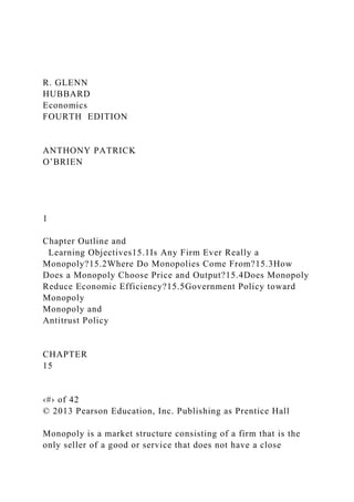
  • 8. 13 A natural monopoly occurs when economies of scale are so large that one firm can supply the entire market at a lower average total cost than can two or more firms. 4. Natural monopoly Figure 15.1 In the market for electricity delivery, a single firm (point A) can deliver electricity at a lower cost than can two firms (point B). This is often because of high fixed costs; in this example, the cost of erecting power lines and transformers, for example. ‹#› of 42 © 2013 Pearson Education, Inc. Publishing as Prentice Hall 14 Explain how a monopoly chooses price and output. 15.3 LEARNING OBJECTIVE How Does a Monopoly Choose Price and Output? ‹#› of 42 © 2013 Pearson Education, Inc. Publishing as Prentice Hall 15
  • 9. In our study of oligopoly, we abandoned the idea of marginal cost and marginal revenue, because the strategic interaction between firms overrode these concepts. Monopolists have no competitors, and hence no concern about strategic interactions. They seek to maximize profit by choosing a quantity to produce, just like perfect and monopolistic competitors. In fact, monopolists act very much like monopolistic competitors: they face a downward sloping demand curve. The difference is that barriers to entry will prevent other firms from competing away their economic profit. The return of marginal cost and marginal revenue ‹#› of 42 © 2013 Pearson Education, Inc. Publishing as Prentice Hall 16 Time Warner Cable is a monopolist in the market for cable television services. The first two columns of the table show the market demand curve, which is also Time Warner’s demand curve. Total, average, and marginal revenue are all calculated in the usual manner. Calculating a monopoly’s revenue ‹#› of 42 © 2013 Pearson Education, Inc. Publishing as Prentice Hall
  • 10. 17 Figure 15.2 As the monopolist seeks to expand its output, two effects occur: Revenue increases from selling an additional unit of output at whatever price is necessary to convince an additional customer to purchase it. Revenue decreases, because the price reduction is shared with existing customers. Graphing a monopoly’s revenue So marginal revenue is always below demand for a monopolist. ‹#› of 42 © 2013 Pearson Education, Inc. Publishing as Prentice Hall 18 Figure 15.3 The monopolist maximizes profit by producing the quantity where the additional revenue from the last unit (marginal revenue) just equals the additional cost incurred from its production (marginal cost). MC = MR determines quantity for a monopolist.
  • 11. Profit-maximizing price and output for a monopoly ‹#› of 42 © 2013 Pearson Education, Inc. Publishing as Prentice Hall 19 Figure 15.3 At this quantity, The demand curve determines price, and The average total cost (ATC) curve determines average cost. Profit is the difference between these (P–ATC), times quantity (Q). Profit-maximizing price and output for a monopoly ‹#› of 42 © 2013 Pearson Education, Inc. Publishing as Prentice Hall
  • 12. 20 Since there are barriers to entry, additional firms cannot enter the market. So there is no distinction between the short run and long run for a monopoly. Then unlike for monopolistic competition, we expect monopolists to continue to earn profits in the long run. Long-run profits ‹#› of 42 © 2013 Pearson Education, Inc. Publishing as Prentice Hall 21 Use a graph to illustrate how a monopoly affects economic efficiency. 15.4 LEARNING OBJECTIVE Does Monopoly Reduce Economic Efficiency? ‹#› of 42 © 2013 Pearson Education, Inc. Publishing as Prentice Hall Suppose that a market could be characterized by either perfect competition or monopoly. Which would be better? The thought experiment here is to suppose there is some market that is perfectly competitive, say the wholesale market for potatoes. Then a single firm buys up all of the potato farms in the country. What would happen to: Price of potatoes? Quantity of potatoes traded?
  • 13. The net benefit of consumers (i.e. consumer surplus)? The net benefit of producers (i.e. producer surplus)? The net benefit of all of society (i.e. economic surplus)? Comparing perfect competition and monopoly ‹#› of 42 © 2013 Pearson Education, Inc. Publishing as Prentice Hall 23 Figure 15.4 The market for potatoes is initially perfectly competitive. Price is PC, quantity traded is QC. Now the market is supplied by a single firm. Since the single firm is made up of all of the smaller firms, the marginal cost curve for this new firm is identical to the old supply curve. If a perfect competition becomes a monopoly… ‹#› of 42 © 2013 Pearson Education, Inc. Publishing as Prentice Hall
  • 14. 24 Figure 15.4 But the new firm maximizes market profit, producing the quantity where marginal cost equals marginal revenue (MC = MR). This quantity (QM) is lower than the competitive quantity (QC). The firm charges the corresponding price on the demand curve, PM. This price is higher than the competitive price, PC. … quantity will fall and price will rise ‹#› of 42 © 2013 Pearson Education, Inc. Publishing as Prentice Hall 25 Fewer potatoes will be traded at a higher price. Consumer surplus will fall (with the higher price).
  • 15. Producer surplus must rise, otherwise the firm would have chosen the perfectly competitive price and quantity. Could the increase in producer surplus offset the decrease in consumer surplus? No! Perfectly competitive markets maximized the economic (total) surplus in a market; if fewer trades take place, the economic surplus must fall. Measuring the efficiency loss from monopoly ‹#› of 42 © 2013 Pearson Education, Inc. Publishing as Prentice Hall 26 With the higher monopoly price, consumer surplus decreases by the areas A+B. Producer surplus falls by C, but rises by A; an overall increase. Area A simply is simply a transfer of surplus: neither inherently good nor bad. But areas B and C are lost surpluses: deadweight loss. Figure 15.5 The inefficiency of monopoly
  • 16. ‹#› of 42 © 2013 Pearson Education, Inc. Publishing as Prentice Hall Recall that a market has productive efficiency if output is produced as cheaply as possible. That is still the case here: the QM units of output are produced at their lowest possible cost. But we lose allocative efficiency: the cost to society of the last unit produced (MCM) is not the same as the benefit to society of the last unit (PM). Figure 15.5 Productive or allocative inefficiency? ‹#› of 42 © 2013 Pearson Education, Inc. Publishing as Prentice Hall There are relatively few monopolies, so the loss of economic efficiency due to monopolies must be relatively small. But many firms have market power: the ability of a firm to charge a price greater than marginal cost. In fact, the only firms that do not have market power are perfectly competitive firms; and perfect competition is rare. Economists estimate that overall, the loss of efficiency in the
  • 17. United States due to market power is probably less than 1% of total U.S. production—about $480 per person annually. Why so low? Most firms face a relatively large degree of competition, resulting in prices much closer to marginal cost than we would see with monopolies. So deadweight loss due to market power is relatively small. How large are these efficiency losses? ‹#› of 42 © 2013 Pearson Education, Inc. Publishing as Prentice Hall 29 Market power may produce some benefit for an economy: the prospect of market power (and the resulting economic profits) drives firms to innovate, creating new products and services. This drive affects large firms—who reinvest profits in the hope of making larger future profits—and small firms—who hope to obtain profits for themselves—alike. The Austrian economist Joseph Schumpeter claimed that this drive would create a “gale of creative destruction” that would eventually benefit consumers more than increased price competition. This helps to explain governmental ambivalence regarding large firms with market power. An argument in favor of market power ‹#› of 42 © 2013 Pearson Education, Inc. Publishing as Prentice Hall
  • 18. 30 Discuss government policies toward monopoly. 15.5 LEARNING OBJECTIVE Government Policy toward Monopoly ‹#› of 42 © 2013 Pearson Education, Inc. Publishing as Prentice Hall In the 1870s and 1880s, several “trusts” had formed: boards of trustees that oversaw the operation of several firms in an industry, and enforced collusive agreements. This helped prompt U.S. antitrust laws, aimed at eliminating collusion and promoting competition among firms. The most important of these laws are detailed below. Antitrust laws and antitrust enforcement Table 15.1LawDate Enacted PurposeSherman Act1890Prohibited “restraint of trade,” including price fixing and collusion. Also outlawed monopolization.Clayton Act1914Prohibited firms from buying stock in competitors and from having directors serve on the boards of competing firms.Federal Trade Commission Act1914Established the Federal Trade Commission (FTC) to help administer antitrust laws.Robinson-Patman Act1936Prohibited firms from charging buyers different prices if the result would reduce competition.Cellar-Kefauver Act1950Toughened restrictions on mergers by prohibiting any mergers that would reduce competition. ‹#› of 42 © 2013 Pearson Education, Inc. Publishing as Prentice Hall
  • 19. 32 The Federal government is particularly concerned about horizontal mergers: mergers between firms in the same industry, as opposed to vertical mergers between two firms at different stages of the production process. Such mergers are likely enhance firms’ market power. The graph shows such a merger, increasing the price from the competitive price (PC) to the monopoly price (PM), and resulting in deadweight loss. Mergers without efficiency gains Figure 15.6 ‹#› of 42 © 2013 Pearson Education, Inc. Publishing as Prentice Hall 33 Firms seeking to merge typically argue that the resulting larger firm will have lower costs, and hence be able to produce more efficiently. Then even if they charge the (new) monopoly price, the result is an improvement for consumers. However, costs may not decrease by as much as the firms claim, resulting in consumers being worse off.
  • 20. Economists with the FTC and Department of Justice review potential mergers one-by-one. Mergers with efficiency gains Figure 15.6 ‹#› of 42 © 2013 Pearson Education, Inc. Publishing as Prentice Hall 34 Economists and lawyers at the Department of Justice and the Federal Trade Commission developed guidelines for themselves and firms to use in evaluating whether potential merger was acceptable. These include: Market definition Measure of concentration Merger standards
  • 21. DOJ and FTC merger guidelines ‹#› of 42 © 2013 Pearson Education, Inc. Publishing as Prentice Hall 35 Suppose Hershey Foods sought to merge with Mars Inc. In what market do these firms compete? The market for candy? The market for snacks? The market for all food? The more broadly defined the market, the smaller (and more harmless) the merger appears. To determine the appropriate scope of the market, the government tries to determine which goods are close substitutes for those produced by the firms. The “appropriate market” is defined as the smallest market containing the firms’ products for which an overall price rise within the market would result in total market profits increasing. (If profits would decrease, there must be adequate substitutes available; hence the market is too narrowly defined.) 1. Market definition ‹#› of 42 © 2013 Pearson Education, Inc. Publishing as Prentice Hall 36 Four-firm concentration ratios (the percentage of industry sales accounted for by the four largest firms) can be useful, but the government seeks a more detailed overall picture of the industry.
  • 22. For this, it uses the Herfindahl-Hirschman Index (HHI), created by squaring the percentage market shares of each firm, and adding up the results. Some examples are given below: 2. Measure of concentrationFirm market sharesFormulaHHI100%100210,00050%, 50%502 + 5025,00030%, 30%, 20%, 20%302 + 302 + 202 + 2022,60010%, 10%, …, 10%10 x 1021,000 ‹#› of 42 © 2013 Pearson Education, Inc. Publishing as Prentice Hall 37 Based on the calculated HHI values, the DOJ and FTC apply the following standards to determine if they ought to challenge the potential merger of two or more firms: Firms having their merger applications challenged must satisfy the DOJ and FTC that their merger would result in substantial efficiency gains. The burden of proof is on the merging firms. 3. Merger standardsIncrease in HHIPost-merger HHI< 100100 – 200> 200< 1,500Challenge unlikelyChallenge
  • 23. unlikelyChallenge unlikely1,500 – 2,500Challenge unlikelyChallenge possibleChallenge possible> 2,500Challenge unlikelyChallenge possibleChallenge very likely ‹#› of 42 © 2013 Pearson Education, Inc. Publishing as Prentice Hall http://www.ftc.gov/os/2010/08/100819hmg.pdf ; see page 19 38 Should AT&T Have Been Allowed to Merge with T-Mobile? Making the Connection In early 2011, AT&T agreed to buy T-Mobile. As the second- and fourth-largest mobile wireless providers in the U.S., this merger would have created a large increase in market concentration: increasing the HHI by over 700 points. The firms claimed that they could operate more efficiently together: closing hundreds of redundant retail stores, and combining their technical and support staff. AT&T estimated cost savings of $3 billion per year. After several months of study, the DOJ filed suit to block the merger, rejecting AT&T’s cost savings estimate. In late 2011, AT&T admitted defeat, and dropped its merger plans. ‹#› of 42 © 2013 Pearson Education, Inc. Publishing as Prentice Hall Natural monopolies have the potential to serve customers more
  • 24. cheaply than multiple firms. But the usual market forces that drive price down do not exist. Local and/or state regulatory commissions typically set prices for these natural monopolies, instead of allowing the firms to set their own price. But that raises the question: what price should the regulators choose? A price that makes the monopoly make zero profit? The efficient price that would maximize consumer welfare? Regulating natural monopolies ‹#› of 42 © 2013 Pearson Education, Inc. Publishing as Prentice Hall 40 Figure 15.7 If the natural monopoly were not subject to regulation, it would choose quantity QM and price PM. Efficiency (MC = MR) suggests a price of QE. But then the firm makes a loss. Regulating natural monopolies
  • 25. The typical compromise is to allow the firm to charge a price where it can make zero economic profit: PR. The resulting quantity QR is hopefully close to the efficient level, keeping deadweight loss small. ‹#› of 42 © 2013 Pearson Education, Inc. Publishing as Prentice Hall 41 Monopoly is a market structure; natural monopoly is a reason the monopoly market structure might exist. Monopolies need not be natural monopolies. No monopolist, not even a natural monopolist, tries to minimize cost. MC = MR guides an (unregulated) monopolist. While our graphs tend to show the efficiency loss from monopolies to be high, estimates of the efficiency loss due to all market power are really quite low: <1% of total output. Common misconceptions to avoid ‹#› of 42 © 2013 Pearson Education, Inc. Publishing as Prentice Hall 42 R. GLENN HUBBARD Economics
  • 26. FOURTH EDITION ANTHONY PATRICK O’BRIEN 1 Firms in Perfectly Competitive Markets CHAPTER 12 Chapter Outline and Learning Objectives12.1Perfectly Competitive Markets12.2How a Firm Maximizes Profit in a Perfectly Competitive Market12.3Illustrating Profit or Loss on the Cost Curve Graph12.4Deciding Whether to Produce or to Shut Down in the Short Run12.5“If Everyone Can Do It, You Can’t Make Money at It”: The Entry and Exit of Firms in the Long Run12.6Perfect Competition and Efficiency ‹#› of 46 © 2013 Pearson Education, Inc. Publishing as Prentice Hall For the next few chapters, we will examine several different market structures: models of how the firms in a market interact with buyers to sell their output. The market structures we will examine are, in decreasing order of competitiveness: Perfectly competitive markets Monopolistically competitive markets Oligopolies, and
  • 27. Monopolies. Each market structure will be applicable to different real-world markets, and will give us insight into how firms in certain types of markets behave. Market structures ‹#› of 46 © 2013 Pearson Education, Inc. Publishing as Prentice Hall 3 Table 12.1Market StructureCharacteristicPerfect CompetitionMonopolistic CompetitionOligopolyMonopolyNumber of firmsManyManyFewOneType of productIdenticalDifferentiatedIdentical or differentiatedUniqueEase of entryHighHighLowEntry blockedExamples of industries• Growing wheat • Growing apples• Clothing stores • Restaurants• Manufacturing computers • Manufacturing automobiles• First-class mail delivery • Tap water The following table identifies the characteristics that determine the type of market. Table of market structures ‹#› of 46 © 2013 Pearson Education, Inc. Publishing as Prentice Hall 4
  • 28. Explain what a perfectly competitive market is and why a perfect competitor faces a horizontal demand curve. 12.1 LEARNING OBJECTIVE Perfectly Competitive Markets ‹#› of 46 © 2013 Pearson Education, Inc. Publishing as Prentice Hall The first market structure we will examine is the perfectly competitive market: one in which There are many buyers and sellers; All firms sell identical products; and There are no barriers to new firms entering the market The first and second conditions imply that perfectly competitive firms are price-takers: they are unable to affect the market price. This is because they are tiny relative to the market, and sell exactly the same product as everyone else. As you might have already guessed, perfectly competitive markets are relatively rare. Introduction to perfectly competitive markets ‹#› of 46 © 2013 Pearson Education, Inc. Publishing as Prentice Hall Figure 12.1 By definition, a perfectly competitive firm is too small to affect the market price. Agricultural markets, like the market for wheat, are often thought to be close to perfectly competitive. Suppose you are a wheat farmer; whether you sell 6,000… … or 15,000 bushels of wheat, you receive the same price per
  • 29. bushel: you are too small to affect the market price. The demand curve for a perfectly competitive firm ‹#› of 46 © 2013 Pearson Education, Inc. Publishing as Prentice Hall 7 There are thousands of individual wheat farmers. Their collective supply, combined with the overall market demand for wheat, determines the market price of wheat. The individual farmer takes this market price as his or her demand curve. How is the firm’s demand curve determined? Figure 12.2 ‹#› of 46 © 2013 Pearson Education, Inc. Publishing as Prentice Hall
  • 30. 8 Explain how a firm maximizes profit in a perfectly competitive market. 12.2 LEARNING OBJECTIVE How a Firm Maximizes Profit in a Perfectly Competitive Market ‹#› of 46 © 2013 Pearson Education, Inc. Publishing as Prentice Hall We assume that all firms try to maximize profits—including perfectly competitive ones. Recall that Profit = Total Revenue – Total Cost Revenue for a perfectly competitive firm is easy to analyze: the firm receives the same amount of money for every unit of output it sells. So Price = Average Revenue = Marginal Revenue This is illustrated in the table on the next slide. Profit maximization as the goal of the firm ‹#› of 46 © 2013 Pearson Education, Inc. Publishing as Prentice Hall Number of Bushels (Q)Market Price (per bushel) (P)Total Revenue (TR)Average Revenue (AR)Marginal Revenue (MR)0 1 2
  • 32. 4 4— $4 4 4 4 4 4 4 4 4 4 Table 12.2 For a firm in a perfectly competitive market, price is equal to both average revenue and marginal revenue. Revenues for a perfectly competitive firm ‹#› of 46 © 2013 Pearson Education, Inc. Publishing as Prentice Hall 11 Quantity (bushels) (Q)Total Revenue (TR)Total Cost (TC) Profit (TR−TC)Marginal Revenue
  • 34. 7.00 7.50 6.50 3.50 −2.00 −10.50— $4.00 4.00 4.00 4.00 4.00 4.00 4.00 4.00 4.00 4.00— $3.00 2.00 1.50 2.00 2.50 3.50 5.00 7.00 9.50 12.50 Table 12.3 Profit maximization as the goal of the firm Suppose costs are as in the table. We can calculate profit; profit is maximized at a quantity of 6 bushels. This is the profit-maximizing level of output.
  • 35. ‹#› of 46 © 2013 Pearson Education, Inc. Publishing as Prentice Hall 12 Quantity (bushels) (Q)Total Revenue (TR)Total Cost (TC) Profit (TR−TC)Marginal Revenue (MR)Marginal Cost (MC)0 1 2 3 4 5 6 7 8 9 10$0.00 4.00 8.00 12.00 16.00 20.00 24.00 28.00
  • 37. 2.00 2.50 3.50 5.00 7.00 9.50 12.50 Table 12.3 Profit maximization as the goal of the firm We can also calculate marginal revenue and marginal cost for the firm. Profit is maximized by producing as long as MR>MC; or until MR=MC, if that is possible. ‹#› of 46 © 2013 Pearson Education, Inc. Publishing as Prentice Hall 13 Figure 12.3a If we show total revenue and total cost on the same graph, the vertical difference between the two curves is the profit the firm makes. (Or the loss, if costs are greater than revenues.) At the profit-maximizing level of output, this (positive) vertical distance is maximized.
  • 38. Showing revenue, cost, and profit ‹#› of 46 © 2013 Pearson Education, Inc. Publishing as Prentice Hall 14 It is generally easier to determine the profit-maximizing level of output on a graph of marginal revenue and marginal cost. Marginal revenue is constant and equal to price for the perfectly competitive firm. The firm maximizes profit by choosing the level of output where marginal revenue is equal to marginal cost (or just less, if equal is not possible). Figure 12.3b Showing marginal revenue and marginal cost ‹#› of 46 © 2013 Pearson Education, Inc. Publishing as Prentice Hall 15
  • 39. The rules we have just developed for profit maximization are: The profit-maximizing level of output is where the difference between total revenue and total cost is greatest; and The profit-maximizing level of output is also where MR = MC. However neither of these rules require the assumption of perfect competition; they are true for every firm! For perfectly competitive firms, we can develop an additional rule, because for those firms, P = MR; this implies: The profit-maximizing level of output is also where P = MC. Rules for profit maximization ‹#› of 46 © 2013 Pearson Education, Inc. Publishing as Prentice Hall Use graphs to show a firm’s profit or loss. 12.3 LEARNING OBJECTIVE Illustrating Profit or Loss on the Cost Curve Graph ‹#› of 46 © 2013 Pearson Education, Inc. Publishing as Prentice Hall We know profit equals total revenue minus total cost; and total revenue is price times quantity. So write: Dividing both sides by Q, we obtain: The “Q”s cancel in the first term, and the second is average total cost; so we can write: Multiplying both sides by Q, we obtain: The right hand side is the area of a rectangle with height (P –
  • 40. ATC) and length Q. We can use this to illustrate profit on a graph. A useful formula for profit ‹#› of 46 © 2013 Pearson Education, Inc. Publishing as Prentice Hall Figure 12.4 A firm maximizes profit at the level of output at which marginal revenue equals marginal cost. The difference between price and average total cost equals profit per unit of output. Showing a profit on the graph Total profit equals profit per unit of output, times the amount of output: the area of the green rectangle on the graph.
  • 41. ‹#› of 46 © 2013 Pearson Education, Inc. Publishing as Prentice Hall 19 Figure 12.4 It is a very common error to believe the firm should produce at Q1: the level of output where profit per unit is maximized. But this does NOT maximize overall profit; the next few units of output bring in more marginal revenue than their marginal cost. Incorrect level of output You can know this because MR>MC at Q1; this demonstrates that Q1 is NOT the profit-maximizing level of output. ‹#› of 46 © 2013 Pearson Education, Inc. Publishing as Prentice Hall 20 We know we should produce at the level of output where marginal cost equals marginal revenue (MC=MR). We have been calling this the profit-maximizing level of output.
  • 42. But what if the firm doesn’t make a profit at this level of output, or at any other? In this case, we would want to make the smallest loss possible. Note that sometimes a loss may be unavoidable, if we have high fixed costs. It turns out that MC=MR is still the correct rule to use; it will guide us to the loss-minimizing level of output. Reinterpreting marginal cost equals marginal revenue ‹#› of 46 © 2013 Pearson Education, Inc. Publishing as Prentice Hall Figure 12.5a In the graph on the left, price never exceeds average cost, so the firm could not possibly make a profit. The best this firm can do is to break even, obtaining no profit but incurring no loss. The MC=MR rule leads us to this optimal level of production. A firm breaking even ‹#› of 46 © 2013 Pearson Education, Inc. Publishing as Prentice Hall 22
  • 43. Figure 12.5b The situation is even worse for this firm; not only can it not make a profit, price is always lower than average total cost, so it must make a loss. It makes the smallest loss possible by again following the MC=MR rule. No other level of output allows the firm’s loss to be so small. A firm making a loss ‹#› of 46 © 2013 Pearson Education, Inc. Publishing as Prentice Hall 23 Once we have determined the quantity where MC=MR, we can immediately know whether the firm is making a profit, breaking even, or making a loss. At that quantity, If P > ATC, the firm is making a profit If P = ATC, the firm is breaking even If P < ATC, the firm is making a loss In fact, these statements hold true at every level of output.
  • 44. Identifying whether or not a firm can make a profit ‹#› of 46 © 2013 Pearson Education, Inc. Publishing as Prentice Hall 24 Explain why firms may shut down temporarily. 12.4 LEARNING OBJECTIVE Deciding Whether to Produce or to Shut Down in the Short Run ‹#› of 46 © 2013 Pearson Education, Inc. Publishing as Prentice Hall Suppose a firm in a perfectly competitive market is making a loss. It would like the price to be higher, but it is a price-taker, so it cannot raise the price. That leaves two options: Continue to produce, or Stop production by shutting down temporarily If the firm shuts down, it will still need to pay its fixed costs. The firm needs to decide whether to incur only its fixed costs, or to produce and incur some variable costs, but obtain some revenue. The firm’s fixed costs should be treated as sunk costs, costs that have already been paid and cannot be recovered, because even if they haven’t literally been paid yet, the firm is still obliged to pay them. Sunk costs should be irrelevant to your decision-making. Responses of perfect competitors to losses ‹#› of 46 © 2013 Pearson Education, Inc. Publishing as Prentice Hall
  • 45. 26 Losing money on Chevy Volts Making the Connection In 2012, Chevrolet was facing intense criticism over its production of the Volt, its small electric/gas hybrid car. Critics pointed out that while Chevrolet sold the Volts for around $40,000, the average total cost of a Volt was around $80,000. But this ATC included large (sunk) fixed costs for research and development; Chevy actually increased profit (decreased loss) by around $15,000 on each additional Volt it sold. Stopping production and sales would have resulted in a larger loss on the Volt than what Chevy actually achieved. Whether it should have initially invested in the hybrid vehicle research that led to the Volt is debatable; but once it had done so, Chevy would have been foolish to stop production just because sales were weaker than they had hoped. ‹#› of 46 © 2013 Pearson Education, Inc. Publishing as Prentice Hall 27 http://www.csmonitor.com/Business/Latest-News- Wires/2012/0910/Plug-in-profit-woes-Chevy-losing-49K-per- Volt-model The firm’s shut down decision is based on its variable costs; it should produce nothing only if: Total Revenue < Variable Cost (P x Q) < VC
  • 46. Dividing both sides by Q, we obtain: P < AVC So if P < AVC, the firm should produce 0 units of output. If P > AVC, then the MC = MR rule should guide production: produce the quantity where MC = MR. For a perfectly competitive firm, this means where MC = P. So the marginal cost curve gives us the relationship between price and quantity supplied: it is the firm’s supply curve! The supply curve of a firm in the short run ‹#› of 46 © 2013 Pearson Education, Inc. Publishing as Prentice Hall 28 Figure 12.6 The firm will produce at the level of output at which MR = MC. Because price equals marginal revenue for a firm in a perfectly competitive market, the firm will produce where P = MC. So the firm supplies output according to its marginal cost curve; the marginal cost curve is the supply curve for the individual firm.
  • 47. The supply curve of a firm in the short run However if the price is too low, i.e. below the minimum point of AVC, the firm will produce nothing at all. The supply is zero below this point. ‹#› of 46 © 2013 Pearson Education, Inc. Publishing as Prentice Hall 29 Figure 12.7 Individual wheat farmers take the price as given… …and choose their output according to the price. The collective actions of the individual farmers determine the market supply curve for wheat. Short run market supply ‹#› of 46 © 2013 Pearson Education, Inc. Publishing as Prentice Hall 30
  • 48. Explain how entry and exit ensure that perfectly competitive firms earn zero economic profit in the long run. 12.5 LEARNING OBJECTIVE “If Everyone Can Do It, You Can’t Make Money at It”: The Entry and Exit of Firms in the Long Run ‹#› of 46 © 2013 Pearson Education, Inc. Publishing as Prentice Hall Explicit CostsWater Wages Fertilizer Electricity Payment on bank loan$10,000 $15,000 $10,000 $5,000 $45,000Implicit CostsForgone salary Opportunity cost of the $100,000 she has invested in her farm$30,000 $10,000Total cost$125,000 Table 12.4 Short-run profit in the carrot-farming industry Sacha starts a small carrot farm, borrowing money from the bank and using some of her savings. Her explicit costs are straight-forward; her implicit costs include the opportunity cost of using her savings, and the salary she gives up to start the farm. Sacha produces 10,000 boxes of carrots each year, and sells them for $15 each. Her total revenue is $150,000. Sacha’s farm makes an economic profit of $25,000 per year. ‹#› of 46 © 2013 Pearson Education, Inc. Publishing as Prentice Hall
  • 49. 32 Economic profit leads to entry of new firms Unfortunately for Sacha, the profits in the carrot-farming business will not last. Why? Additional firms will enter the market, attracted by the profit. Perhaps: Some farms will switch from other produce to carrots, or People will open up new farms However it happens, the number of firms in the market will increase, increasing supply; this will in turn lower the price Sacha can receive for her output. ‹#› of 46 © 2013 Pearson Education, Inc. Publishing as Prentice Hall 33 Figure 12.8 Sacha Gillette’s costs are given in the panel on the right. The price of output is determined by the market, on the left. Sacha makes an economic profit when the price is $15. The profit attracts new firms, which increases supply.
  • 50. The effect of entry on economic profit ‹#› of 46 © 2013 Pearson Education, Inc. Publishing as Prentice Hall 34 The effect of entry on economic profit—continued Figure 12.8 The increased supply causes the market equilibrium price to fall. It falls until there is no incentive for further firms to enter the market; that is, when individual farmers make no economic profit. For this to be true, the price must be equal to ATC; but since P=MC, that means all three must be equal.
  • 51. ‹#› of 46 © 2013 Pearson Education, Inc. Publishing as Prentice Hall 35 Figure 12.9a-b Price is $10 per box, and carrot-farmers are breaking even. Then demand for carrots falls. Price falls to $7 per box. Sacha can no longer make a profit; she makes the smallest loss possible by producing 5000 carrots: where MC = MR. The effect of economic losses ‹#› of 46 © 2013 Pearson Education, Inc. Publishing as Prentice Hall 36 Discouraged by the losses, some firms will exit the market. The resulting decrease in supply causes prices to rise. Firms continue to leave until price returns to the break-even
  • 52. price of $10 per box. Figure 12.9c-d The effect of economic losses ‹#› of 46 © 2013 Pearson Education, Inc. Publishing as Prentice Hall 37 Long-run equilibrium in a perfectly competitive market The previous slides have described how long-run equilibrium is achieved in a perfectly competitive market: If firms are making an economic profit, additional firms enter the market, driving down price to the break-even level. If firms are making an economic loss, existing firms exit the market, driving price up to the break-even level. Since the long-run average cost curve shows the lowest cost at which a firm is able to produce a given quantity of output in the long run, we expect price to be driven down to the typical
  • 53. firm’s long-run average cost curve. Long-run competitive equilibrium: The situation in which the entry and exit of firms has resulted in the typical firm breaking even. ‹#› of 46 © 2013 Pearson Education, Inc. Publishing as Prentice Hall 38 Long-run supply in a perfectly competitive market This means that in the long run, the market will supply any demand by consumers at a price equal to the minimum point on the typical firm’s average cost curve. Hence the long-run supply curve is horizontal at this price. In a perfectly competitive market, the long-run price is completely determined by the forces of supply. The number of suppliers adjusts to meet demand, at the lowest possible price. Long-run supply curve: A curve that shows the relationship in the long run between market price and the quantity supplied. ‹#› of 46 © 2013 Pearson Education, Inc. Publishing as Prentice Hall 39
  • 54. Figure 12.10 The panels show how an increase or decrease in demand is met by a corresponding increase or decrease in supply. Price always returns to the long-run (break-even) level. Long-run supply in a perfectly competitive market ‹#› of 46 © 2013 Pearson Education, Inc. Publishing as Prentice Hall 40 Increasing-cost and decreasing-cost industries Industries where the production process is infinitely replicable are modeled well by this horizontal supply curve. But what if this is not the case? If some factor of production cannot be replicated, additional firms may have higher costs of production. Example: If certain grapes grow well only in certain climates, then the cost to produce additional grapes may be higher than
  • 55. for existing firms. On the other hand, sometimes additional firms might generate benefits for other firms in the market, leading additional firms to have lower costs of production. Example: Cell phones require specialized processors. As more firms produce cell phones, economies of scale in processor- production reduce cell phone costs. ‹#› of 46 © 2013 Pearson Education, Inc. Publishing as Prentice Hall 41 Economic profits are rapidly competed away in the iPhone apps store. In the Apple iPhone Apps Store, Easy Entry Makes the Long Run Pretty Short Making the Connection When firms earn economic profits in a market, other firms have a strong economic incentive to enter that market. This is exactly what happened with iPhone apps, first provided for Apple in mid-2008. Proving to be highly profitable in an instant, more than 25,000 apps were available in the iTunes store within a year. The cost of entering this market was very small. Anyone with the programming skills and the time to write an app could have it posted in the store. As a result of this enhanced competition, the ability to get rich quick with a killer app fades quickly. ‹#› of 46
  • 56. © 2013 Pearson Education, Inc. Publishing as Prentice Hall 42 Explain how perfect competition leads to economic efficiency. 12.6 LEARNING OBJECTIVE Perfect Competition and Efficiency ‹#› of 46 © 2013 Pearson Education, Inc. Publishing as Prentice Hall Types of efficiency Efficiency in economics really refers to two separate but related concepts: Productive efficiency is a situation in which a good or service is produced at the lowest possible cost. Allocative efficiency is a state of the economy in which production represents consumer preferences; in particular, every good or service is produced up to the point where the last unit provides a marginal benefit to consumers equal to the marginal cost of producing it. ‹#› of 46 © 2013 Pearson Education, Inc. Publishing as Prentice Hall 44 Are perfectly competitive markets efficient?
  • 57. We have shown that in the long run, perfectly competitive markets are productively efficient. But they are allocatively efficient also: The price of a good represents the marginal benefit consumers receive from consuming the last unit of the good sold. Perfectly competitive firms produce up to the point where the price of the good equals the marginal cost of producing the good. Therefore, firms produce up to the point where the last unit provides a marginal benefit to consumers equal to the marginal cost of producing it. Productive and allocative efficiency are useful benchmarks against which to measure the actual performance of other markets. ‹#› of 46 © 2013 Pearson Education, Inc. Publishing as Prentice Hall 45 Common misconceptions to avoid While a perfectly competitive firm faces a horizontal demand curve, the market demand curve is still “normal” (downward- sloping). In this chapter there are many supply curves described: the individual firm’s supply curve, the market short-run supply curve, the market long-run supply curve; do not confuse these. Remember that “zero economic profit” is an adequate level of profit to cover opportunity costs; it is not a bad outcome for a firm.
  • 58. The reasons for shutting down in the short run and exiting the market in the long run are different: P<AVC for the short run, P<ATC for the long run. ‹#› of 46 © 2013 Pearson Education, Inc. Publishing as Prentice Hall 46 TC Q P - ´ = ) ( Profit Q TC Q Q P - ´ = ) ( Q Profit ATC P - = Q