Downloaded 1,271 times


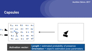
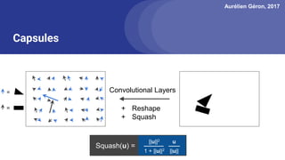
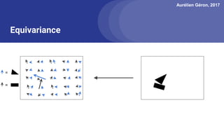
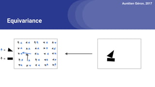

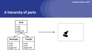

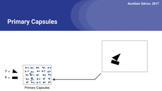
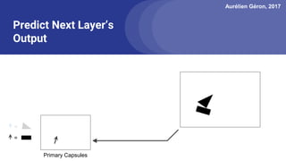
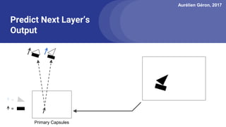
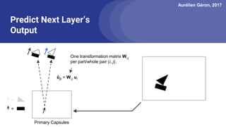

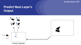
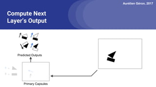
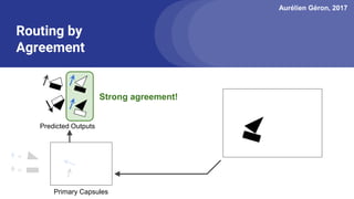
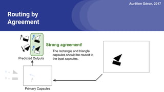
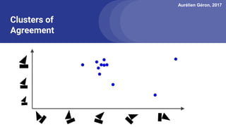
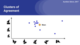
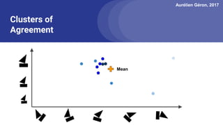


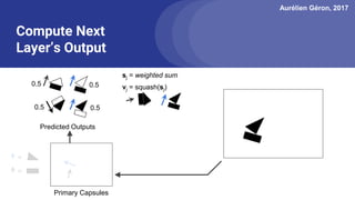
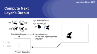
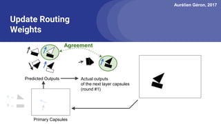

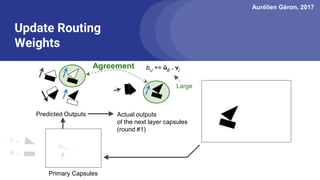
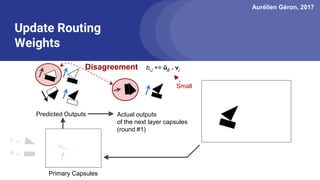
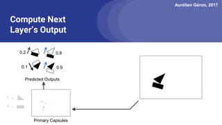


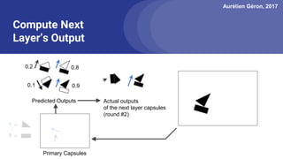
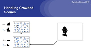
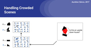
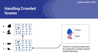
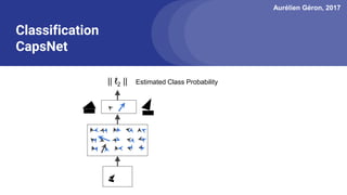
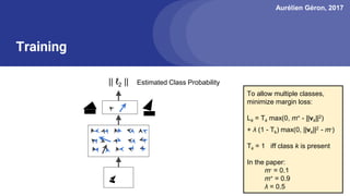
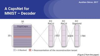

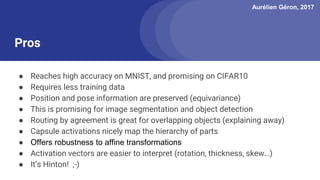
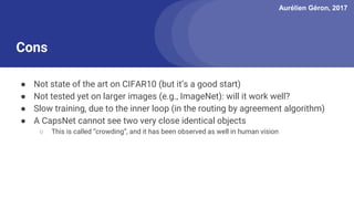
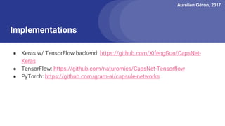


The document discusses capsule networks, focusing on their architecture and functionality, including dynamic routing, activations, and handling of perspective transformations. It highlights the advantages of capsule networks, such as high accuracy on MNIST and robustness to affine transformations, while also addressing limitations like slow training and issues with closely clustered objects. Additionally, it provides links to various implementations and resources related to capsule networks.


![[PR12] Capsule Networks - Jaejun Yoo](https://cdn.slidesharecdn.com/ss_thumbnails/pr12capsulenetworks-jaejunyoo-171217144319-thumbnail.jpg?width=640&height=640&fit=bounds)


![[Paper] dynamic routing between capsules](https://cdn.slidesharecdn.com/ss_thumbnails/paperdynamicroutingbetweencapsules-210509101120-thumbnail.jpg?width=640&height=640&fit=bounds)


![제 23회 보아즈(BOAZ) 빅데이터 컨퍼런스 - [MBOAX] : ABSA를 활용한 소비자 반응 분석 기반 운영 효율화 대시보드 설계](https://cdn.slidesharecdn.com/ss_thumbnails/3-1boaz23rdconferencemboax-260203102709-9d519923-thumbnail.jpg?width=640&height=640&fit=bounds)


