BBA 2401, Principles of Macroeconomics 1 Learning Obj.docx

BBA 2401, Principles of Macroeconomics 1
Learning Objectives
Upon completion of this unit, students should be able to:
1. Describe the relationship between the demand and supply of
money.
2. Explain how changes in the money supply affect aggregate
demand in
the short run.
3. Explain how changes in the money supply affect aggregate
demand in
the long run.
4. Evaluate targets for monetary policy.
5. Compare an active policy and a passive policy.
6. Explain the Phillips curve.
Written Lecture
Monetary theory is concerned with the effects of the quantity of
money on the
economy's price level and the level of real output. There is
considerable debate
among economists concerning what these effects are. One
difficulty in

determining the effects is that monetary policy changes and
fiscal policy
changes often occur at the same time, so it is difficult to sort
out the effects of
one from those of the other. This chapter describes two views of
how money
affects the economy: a short-run view and a long-run view.
The Demand and Supply of Money
A person's demand for money is not the same as the person's
desire for a
greater income. When economists speak of a demand for money,
they are
referring to the desire to hold a particular amount of money,
either in checking
accounts or as cash. That is, the demand for money is a demand
to hold a
stock of money at a particular time. Since money is used to
facilitate exchange
of goods and services and people engage in exchange on a
regular basis,
people hold money balances. The demand for money is greater
the greater the
number of transactions (as measured by real GDP) and the
higher the average
price at which each good is sold, that is, the greater nominal
GDP.
Money also competes with other financial assets as a store of
wealth.
Compared with other financial assets, money has one major
advantage and
one major disadvantage. Money's advantage is its liquidity—it
can be directly
exchanged for goods and services. Its disadvantage is that it

earns either no
interest or substantially less interest than other financial assets.
The
opportunity cost of holding money is the additional interest that
could have
been earned by using the money to buy alternative interest-
bearing financial
assets. Consequently, the cost of holding money increases with
the real
interest rate, and we expect the demand for money to vary
inversely with the
real interest rate, other things being constant. That is, the
demand curve for
money slopes downward when real interest rates are on the
vertical axis.
Reading
Assignments
Chapter 16:
Monetary Theory and
Policy
Chapter 17:
Macro Policy Debate:
Active or Passive?
Supplemental
Reading
Click here to access a
PDF of the Chapter 16
Presentation.

Click here to access a
PDF of the Chapter 17
Presentation.
Learning Activities
(Non-Graded)
See information below.
Key Terms
1. Decision-making lag
2. Demand for money
3. Effectiveness lag
4. Equation of exchange
5. Implementation lag
6. Long-run Phillips
curve
7. Natural rate
hypothesis
8. Phillips curve
9. Quantity theory of
money
10. Rational expectations
UNIT VII STUDY GUIDE
Monetary Theory and Macro Policy

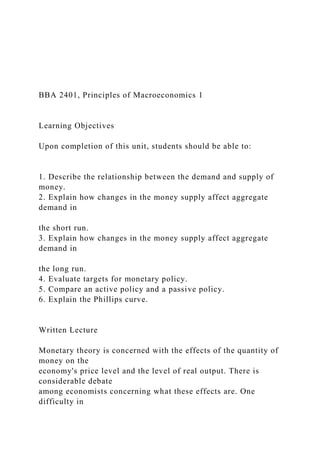
http://online.columbiasouthern.edu/CSU_Content/Courses/Busin
ess/BBA/BBA2401/12M/UnitVII_Chapter16Presentation.pdf
http://online.columbiasouthern.edu/CSU_Content/Courses/Busin
ess/BBA/BBA2401/12M/UnitVII_Chapter17Presentation.pdf
The supply of money in the economy is determined primarily by
the Fed, so we
make the simplifying assumption that the quantity of money
supplied is
constant no matter what the interest rate is. Hence, the supply
curve for money
is a vertical line at whatever quantity of money the Fed has
determined.
Exhibit 1 illustrates the money market. The demand for money
slopes down, as
mentioned, and the supply curve for money is perfectly
inelastic. Suppose that
the supply of money is indicated initially by supply curve S.
The intersection of
the two curves determines the equilibrium interest rate, 10
percent. An
increase in the supply of money shifts the supply curve to S´
and generates a
lower equilibrium interest rate, 6 percent; an increase in the
demand for money
generates a higher interest rate.

Money and Aggregate Demand in the Short Run
If money is to affect aggregate demand, it must do so by
affecting one of
several things: consumption spending, investment spending,
government
spending, or net exports. As we have just seen, changes in the
supply of
money cause changes in interest rates. In the model that
emphasizes the short
run then, monetary policy affects aggregate demand indirectly
by influencing

the market rate of interest, which affects the level of planned
investment.
Suppose the Fed wants to pursue a tight monetary policy and
reduce the
supply of money. The Fed can reduce the money supply by
raising the
discount rate, selling government securities, or raising the
required reserve
ratio. Regardless of which method is used, the money supply
curve shifts to the
left and the market rate increases. In Exhibit 2, the higher
interest rate causes
a movement along the demand curve for investment and the
level of
investment falls. As a result, aggregate demand shifts to the
left, as shown in
Exhibit 3.
(McEachern, W. A., 2012)
11. Recognition lag
12. Short-run Phillips
curve
13. Time-inconsistency
problem
14. Velocity of money

The shifts in the curves in Exhibit 3 are not the end of the story.
The aggregate
supply curve slopes upward, so the ultimate effects of a change
in the money
supply are partially determined by the shape of the aggregate
supply curve.
Exhibit 4 shows the bottom part of Exhibit 3 with a short-run
aggregate supply
curve added. At the original price level, 100, there is an excess
supply after the
aggregate demand curve shifts from AD to AD´. The excess
supply causes
prices to fall until equilibrium is reached at price level 90 and
real GDP of
$4 trillion. Thus, the reduction of the money supply has
generated a reduced
level of GDP and a lower price level.

Money and the Aggregate Demand in the Long Run
Monetarists use the equation of exchange to analyze the effects
of changes in
the money supply. Monetarists argue that an increase in the
money supply
leaves individuals with larger money balances than they desire.
Individuals
reduce their money balances by increasing their spending on all
goods, not just
other financial assets. The increased spending on all goods has a
direct effect
on aggregate demand.

The equation of exchange is a tautology—that is, it is true by
definition.
Nominal income equals real output, Y, times the price level, P.
Since money is
used in exchange, nominal income must be equal to the quantity
of money in
the economy, M, multiplied by the average number of times per
year money
changes hands to purchase final goods and services, V. Hence,
M x V = P x Y.
The average number of times money changes hands in a year, V,
is called
the velocity of money. The quantity theory of money states that
velocity is
predictable and stable. Consequently M = (P x Y)/V, and
changes in the money
supply cause predictable changes in nominal income. Whether
the change in
nominal income is due to changes in the price level or to
changes in real output
depends on the shape of the aggregate supply curve. In the short
run, the
aggregate supply curve slopes upward, so an increase in
aggregate demand
induced by an increase in the supply of money leads to
increased real output

and higher prices. In the long run, the aggregate supply curve is
vertical, and
an increase in aggregate demand leads only to an increase in the
price level.
Those who focus on the short-run effects of monetary policy do
not accept the
monetarist belief that velocity is stable. Instead, they believe
that velocity varies
with the interest rate. According to this view, an increase in the
interest rate
increases the opportunity cost of holding money, so the quantity
of money held
falls and the velocity of money rises. To the extent that a
change in interest
rates affects velocity, changes in the money supply are offset by
changes in
velocity.
Targets for Monetary Policy
Given the differences in their views of the effects of money on
the economy, it
should not be surprising that the policy prescriptions of those
who focus on the
short run differ from the prescriptions of those who focus on the
long run. The
first group argues that monetary policy should focus on interest
rates.
Monetarists believe that money has a more direct effect on
nominal income, so
they argue that monetary authorities should focus more on
money supply
targets. For most of the postwar period, monetary authorities
have focused on
interest-rate targets rather than on monetary growth-rate targets.

In recent
years there have been large movements of funds into and out of
the United
States in response to interest-rate differentials between the
United States and
other countries. These flows affect the exchange rate and the
level of imports
and exports. Consequently, the Fed has been forced to give
greater
consideration to the international effects of its monetary policy
decisions.
Active Policy Versus Passive Policy
The federal government is very concerned with economic policy
questions. The
Employment Act of 1946 makes the federal government
responsible for
maintaining full employment. Even without such a law,
politicians would be
interested in economic policy. Incumbents find it easier to be
reelected when
the economy is functioning well than when inflation is high and
rising, or
unemployment rates are high. Thus, the question of interest is
which policy is
the best policy. Unfortunately for policymakers, the answer to
the question
remains unclear, and the topic is hotly debated among
economists.
Some economists advocate an active role for the federal
government. An
active policy is one in which policymakers make use of
discretionary
stabilization policies to keep the economy running at or near

potential output
while maintaining relatively stable prices. Discretionary fiscal
and monetary
policies tend to focus on shifting the aggregate demand curve to
achieve full
employment. An expansionary monetary policy is used to
stimulate spending
when real GDP is below potential, and a restrictive monetary
policy is used to
reduce spending when the economy is overheated. Fiscal policy
can also be
used to stimulate or reduce aggregate demand. Advocates of an
active policy
tend to argue that the private economy is basically unstable and
private
spending cannot be counted upon to maintain aggregate demand
at the full
employment level. According to this view, by implementing the
correct
discretionary policies the government can stabilize the economy
around
potential output.
Other economists disagree and advocate a passive role for the
government.
They believe the private economy is inherently stable and self-
correcting.
Deviations from potential GDP tend to be short-lived because
self-correcting
market forces push the economy toward its potential output.
Since the
economy is basically stable, there is no need for discretionary
stabilization
policy. In fact, according to this view, government stabilization
policies are
inherently destabilizing because there are various time lags

between the
recognition of a problem, the selection and implementation of a
policy to
correct it, and the impact of a policy change on the economy.
During the time
lags, the economy's self-correcting mechanisms return the
economy to its full
employment level. Consequently, when the discretionary policy
takes effect, it
may generate a new problem, since the problem it was designed
to alleviate
has already corrected itself.
Role of Expectations
Individuals make economic decisions on the basis of their
experiences; the
information they have about prices, inflation, and the like; and
their
expectations, which are based on information about future
economic
conditions. This information comes from many sources. For
example, a
possible change in government tax policy is discussed and
debated in public
for a considerable time before it is implemented. Money supply
figures are
published regularly, as are unemployment rates and numerous

other measures
of economic activity.
By affecting short-run aggregate supply, the expectations of
economic actors
play a crucial role in determining whether a particular
discretionary policy will
be effective. The rational expectations school of thought holds
that people form
expectations on the basis of all relevant information, including
information
about how government stabilization policy operates and is
implemented.
Consequently, if policymakers attempt to stimulate the economy
by increasing
the rate of growth of the money supply and people correctly
anticipate that the
Fed is going to do this, then the monetary growth will not have
any short-run
effect on output. Instead, the only effect will be a long-run
increase in the
inflation rate.

Exhibit 1 illustrates the views of the rational expectations
school. Potential
output is $5 trillion, and the current equilibrium is at e*.
Suppose the Fed
announces a restrictive monetary policy in an effort to reduce
the price level to
95, and it initially pursues the restrictive monetary policy.
Aggregate demand
shifts to AD´, real GDP falls to $4 trillion, and the price level
falls to 100. Once
the public perceives the new conditions and they adjust their
decisions about
supplying resources in the light of their new information, the
short-run

aggregate supply curve shifts to SRAS(95), and the new long-
run equilibrium is
at e´. Suppose, however, that the Fed abandons its restrictive
monetary policy
before the public adjusts its price expectations to 95. If the
public is unaware of
this change, aggregate demand returns to AD* at the same time
that the short-
run aggregate supply curve shifts to SRAS(95), and real GDP
increases to
$6 trillion. The public gets caught by surprise. Eventually,
people will realize
the true state of the economy, and the short-run aggregate
supply will shift
back to SRAS(105).
By failing to implement its announced policy, the Fed loses its
credibility with
the public. If the Fed now announces a restrictive monetary
policy to combat
inflation, the public will be less likely to believe the
announcement.
Consequently, people will not change their price expectations,
and the short-
run aggregate supply curve will not shift. The Fed would have
to pursue its
restrictive monetary policy for a longer period of time to
convince the public that
it was serious. During this time, however, real GDP would be
below potential
output, and unemployment would be above the natural rate of
unemployment.
Policy Rules Versus Discretion
Since advocates of a passive policy believe the government's

use of
discretionary policy tends to destabilize the economy, they
advocate the use of
monetary policy rules. A monetary policy rule specifies the
relationship
between a policy instrument and a policy objective. Some
economists support
rules on the grounds that the government cannot effectively
control the
economy because it is so complex and the lags involved in
discretionary
policies are too long and variable. Those who favor the rational
expectations
approach advocate rules because they believe the public is
sophisticated
enough in forming its expectations that discretionary policy
tends to affect only
the level of prices. By making policy on the basis of a rule, the
Fed makes it
possible for the public to formulate expectations about the
future with greater
certainty and permits the economy to achieve the natural rate of
output.
The Phillips Curve
The Phillips curve is a graphical representation of a tradeoff
between inflation
and unemployment. The tradeoff shown by a Phillips curve is
between low
unemployment rates and low inflation rates; it is not possible to
have both. That
is, if the government wants to lower the unemployment rate, it
must be willing
to accept a higher inflation rate. Exhibit 2 illustrates two
possible Phillips

curves. During the 1960s, policymakers acted on the belief that
there was a
stable, long-run tradeoff between inflation and unemployment
for the economy.
As inflation became a greater problem in the late 1960s and
early 1970s,
however, this view became suspect. Critics of an active policy
argued that the
tradeoff is a short-run, not a long-run, phenomenon. According
to this view, the
government may be able to trade greater inflation for lower
unemployment in
the short run. Once the public realizes the true state of the
economy, however,
unemployment will return to its natural rate. In Exhibit 2, the
natural rate of
unemployment is 6 percent. Suppose the economy is at point a.
The
government can temporarily reduce unemployment by creating
inflation; in that
case, the economy moves to point b. Once the public perceives
the new
economic situation, people adjust their expectations, and the
economy returns
to the natural rate of unemployment (point c). Now the natural
rate of
unemployment is associated with a higher inflation rate, and
there is a new
short-run Phillips curve. The long-run Phillips curve is vertical
at the natural
rate of unemployment.

Learning Activities (Non-Graded)
Click on the following link to watch a video on Inflation and
the Money Supply:
http://www.swlearning.com/economics/abcvideos/TMG0005160
1.html
Non-graded learning activities are provided to aid students in
their course of
study. This is a non-graded activity, so you do not have to
submit it.
http://www.swlearning.com/economics/abcvideos/TMG0005160
1.html

BBA 2401, Principles of Macroeconomics 1 Learning Obj.docx

Recommended

Recommended

More Related Content

Similar to BBA 2401, Principles of Macroeconomics 1 Learning Obj.docx

Similar to BBA 2401, Principles of Macroeconomics 1 Learning Obj.docx (20)

More from arnit1

More from arnit1 (20)

Recently uploaded

Recently uploaded (20)

BBA 2401, Principles of Macroeconomics 1 Learning Obj.docx