Download as PDF, PPTX

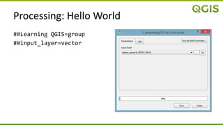
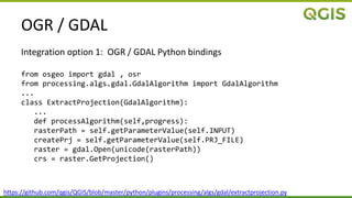
![OGR / GDAL
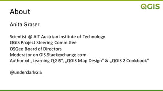
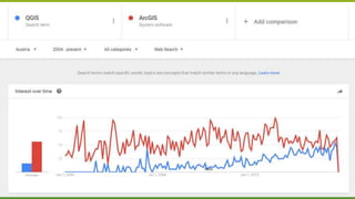
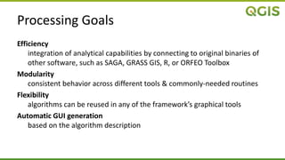
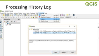
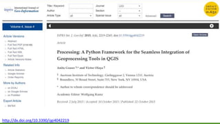
Integration option 2: command line interface using Python’s subprocess
from processing.algs.gdal.GdalAlgorithm import GdalAlgorithm
from processing.algs.gdal.GdalUtils import GdalUtils
...
class ClipByExtent(GdalAlgorithm):
...
def processAlgorithm(self, progress):
out = self.getOutputValue(self.OUTPUT)
...
arguments = []
arguments.append(’-of’)
arguments.append(GdalUtils.getFormatShortNameFromFilename(out))
...
GdalUtils.runGdal([’gdal_translate’, GdalUtils.escapeAndJoin(arguments)],
progress)
https://github.com/qgis/QGIS/blob/master/python/plugins/processing/algs/gdal/ClipByExtent.py](https://image.slidesharecdn.com/processing2017-170505154501/85/QGIS-Processing-at-Linuxwochen-Wien-PyDays-2017-21-320.jpg)
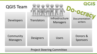
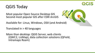
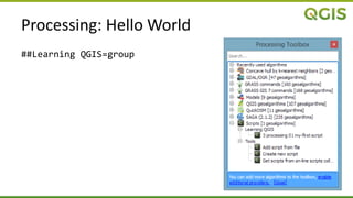
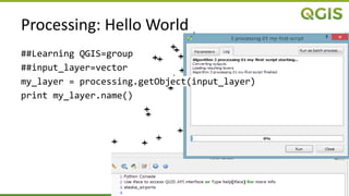
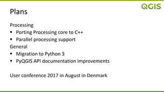
![R
Standard R syntax
Extended by additional header elements
##Vector processing=group
##showplots
##Layer=vector
##Field=Field Layer
hist(Layer[[Field]], main=paste("Histogram of",Field),
xlab=paste(Field))](https://image.slidesharecdn.com/processing2017-170505154501/85/QGIS-Processing-at-Linuxwochen-Wien-PyDays-2017-24-320.jpg)
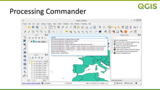
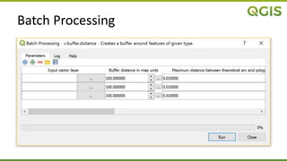
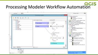

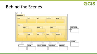
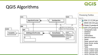
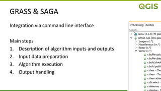
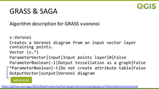
QGIS is an open source desktop GIS that is the second most popular GIS after ESRI ArcGIS. It has been in development since 2002 and integrates geoprocessing tools using Python. The Processing plugin allows users to run algorithms from other software like SAGA and GRASS through Python scripts. These scripts handle tasks like describing algorithms, preparing input data, executing processes, and managing outputs. The plugin also supports batch processing, workflows, and accessing algorithms from R. Future plans include porting Processing to C++ and adding parallel processing support.


![[FOSS4G Seoul 2015] New Geoprocessing Toolbox in uDig Desktop GIS](https://cdn.slidesharecdn.com/ss_thumbnails/foss4g2015newgeoprocessingtoolboxinudigdesktopapplicationframework-150917042904-lva1-app6892-thumbnail.jpg?width=640&height=640&fit=bounds)


