The history of radar began in the late 19th century with Maxwell's theory of electromagnetism and Hertz's experiments verifying the existence of radio waves that could reflect off objects. Early pioneers included Hülsmeyer who invented the first radar system in 1904 and Marconi who recognized its potential for ship detection. During the 1930s, radar was independently developed by several countries including the US, UK, Germany and others. The UK played a key role with Watson-Watt demonstrating radar detection of aircraft at Daventry in 1935. This led to the development of pulse radar and the Chain Home radar network which helped defend Britain in WWII. Germany also made major advances with naval and airborne radar including the Freya,

1. Peter Devine
Peter Devine
Radar level
measurement
Radar level measurement
Radar level measurement The user's guide
The user's guide

2. Radar level measurement
- The users guide
Peter Devine
written by
Peter Devine
additional information
Karl Grießbaum
type setting and layout
Liz Moakes
final drawings and diagrams
Evi Brucker
© VEGA Controls / P Devine / 2000
All rights reseved. No part of this book may reproduced in any way, or by any means, without prior
permissio in writing from the publisher:
VEGA Controls Ltd, Kendal House, Victoria Way, Burgess Hill, West Sussex, RH 15 9NF England.
British Library Cataloguing in Publication Data
Devine, Peter
Radar level measurement - The user´s guide
1. Radar
2. Title
621.3´848
ISBN 0-9538920-0-X
Cover by LinkDesign, Schramberg.
Printed in Great Britain at VIP print, Heathfield, Sussex.

3. Contents
Foreword
Acknowledgement
Introduction
ix
xi
xiii
Part I
1. History of radar
2. Physics of radar
3. Types of radar
1. CW-radar
2. FM - CW
3. Pulse radar
1
13
33
33
36
39
Part II
4. Radar level measurement
1. FM - CW
2. PULSE radar
3. Choice of frequency
4. Accuracy
5. Power
47
48
54
62
68
74
5. Radar antennas
1. Horn antennas
2. Dielectric rod antennas
3. Measuring tube antennas
4. Parabolic dish antennas
5. Planar array antennas
Antenna energy patterns
77
81
92
101
106
108
110
6. Installation
A. Mechanical installation
1. Horn antenna (liquids)
2. Rod antenna (liquids)
3. General consideration (liquids)
4. Stand pipes & measuring tubes
5. Platic tank tops and windows
6. Horn antenna (solids)
B. Radar level installation cont.
1. safe area applications
2. Hazardous area applications
115
115
115
117
120
127
134
139
141
141
144

4. Foreword
To suggest that any one type of level
transmitter technology could be regarded as 'universal' would be unrealistic
and potentially irresponsible due to the
variation and complexity of available
applications when liquids, powders and
solids are all considered. However, the
rate at which radar based level transmitters have established themselves
over the last couple of years would
tend to suggest that this technology is
closer to that definition that any principle has ever been.
I have personally been involved in
the development, applications, sales
and marketing of level transmitters,
controllers and indicators of most types
over the last twenty years. In that time
nothing has, in my opinion, come close
to matching the significance of radar in
terms of its overall suitability, for not
just conventional but extreme process
conditions applications for the vast
majority of substances in vessels of virtually any size or complexity.
This unique principle combined with
current reflections processing software,
materials of construction, simplicity of
installation and transmitter digital communications allows this to be considered as a day to day 'first consideration'
for level, whereas only a very short
time ago it was regarded as expensive
and specialised - this is no longer the
case.
The purpose of this publication is
quite specific, and that is to explain
some of the principles involved, and to
show that by applying some simple
guidelines, what is obviously a sophisti-cated technology can be simple and
reliably used in an enormously wide
range of industrial and process applications.
We make no apology for including a
chapter on Vega specific products, and
hope this guide stimulates a radar user,
or some greater depth of knowledge if
you have some experience, we look
forward to hearing from you.
Mel Henry
Managing Director
Vega Controls Ltd.
ix

5. Acknowledgements
In writing and compiling this book I
had the invaluable assistance of several
colleagues from VEGA in Schiltach
both in the developing department and
within the product management.
Particular thanks must go to Karl
Griessbaum for his lucid explanations
of the 'secrets' of pulse radar; his insight into the workings of FM - CW
radar and the drawings to accompany
the explanations. Thanks also to
Juergen Skowaisa and Juergen Motzer
for their technical contributions to the
book.
The publication of 'radar level measurement - the user´s guide' is a reflection of the wealth of product knowledge of radar level application experience
in the VEGA group of companies and
our agents and distributors world wide.
This experience has accelerated
since the advent of the VEGAPULS 50
series two wire, loop powered radar.
I would like to thank all those who
contributed to the section on radar
applications. This in-cludes Doug
Anderson, Dave Blenkiron, Chris
Brennan, Graeme Cross and John
Hulme in the UK, Paal Kvam of
Hyptech in Norway, Dough Groh and
his colleagues at Ohmart VEGA in the
USA, and Juergen Skowaisa and Roger
Ramsden from VEGA Germany. Thank
also to the VEGA marketing department in Germany and the UK for their
assistance in producing and collating
pictures and photographs.
Thank to all the other unnamed contributors.
Finally, the most important contributors to this book are all VEGA radar
users world wide without whom our
high level of expertise in process radar
measurement applications would not be
possible.
Peter Devine
Technical manager
Vega Controls Ltd.
xi

6. Introduction
The technical benefits of radar as a
level measurement technique are clear.
Radar provides a non-contact sensor
that is virtually unaffected by changes
in process temperature, pressure or the
gas and vapour composition within a
vessel.
In addition, the measurement accuracy is unaffected by changes in density, conductivity and dielectric constant
of the product being measured or by air
movement above the product.
These benefits have become more
significant to the process industry since
the advent of low costs, high performance, two wire loop powered radar
level transmitters.
This breakthrough, in the summer of
1997, produced an unprecedented
boom in the use of non-contact microwave radar transmitters for liquid and
solids process level application.
'Radar level measurement - the
user´s guide' is offered as a reference
book for all those interested in the technology, the application, and the practical installation of radar level sen-sors.
We cover many practical process level
applications rather than the closed
niche market of custody transfer measurement.
Radar history, physics and techniques are presented as well as descriptions of types of ra-dar antenna and
mechanical and electrical installations.
Now radar is an affordable option
for process level measurement. We
compare it closely with all of the other
process level techniques and give many
examples of the myriad applications of
radar across all industries.
Radar level measurement has come
of age. We hope that this book will be
invaluable in helping you to see the
potential of this latest and almost universal level measurement technology.
More than anything, we hope that
you enjoy delving into the pages of this
book.
Peter Devine
Technical manager
Vega Controls Ltd
xiii

7. 1. History of radar
James Clerk Maxwell predicted the
existence of radio waves in his theory
of electromagnetism as long ago as
1864. He showed mathematically that
all electromagnetic waves travel at the
same velocity in free space,
independent of their wavelength. This
velocity is of the order of 300,000 kilometres per second, the speed of light.
Heinrich Rudolf Hertz, verified
Maxwell’s theory by experiments carried out in 1886-87 at Karlsruhe
Polytechnic. He used a spark gap transmitter producing bursts of high frequency electromagnetic waves at about
455 MHz, or a wavelength of 0.66
metres.
Hertz confirmed that these electromagnetic radio waves had the same
velocity as light and could be reflected
by metallic and dielectric bodies. In
addition to their reflective properties,
Hertz demonstrated that radio waves
exhibit refraction, diffraction, polarization and interference in the same way
as light. These early experiments in
reflecting radio waves off metal plates
were the first manifestations of radar as
we know it today.
The first practical form of radar was
produced by a German engineer,
Christian Hülsmeyer. Patented in various countries in 1904 as the
‘Telemobiloscope’, Hülsmeyer’s apparatus was described as ‘A Hertzian
wave projecting and receiving apparatus adapted to indicate or give
warning of the presence of a metallic
body, such as a ship or a train, in the
line of projection of such waves’.
An addition to the patent in the same
year described ‘Improvements in
Hertzian wave projecting and receiving
James Clerk Maxwell predicted the existence of radio waves in
his theory of electromagnetism
(Pic. 1.1 - J.C.M.F)
Heinrich Hertz Hertz confirmed by experiment that electromagnetic radio waves have the same
velocity as light and can be reflected by
metallic and dielectric bodies
(Pic. 1.2 - I.N.T)
1

8. Prior to World War II, radar was
being developed independently in a
number of different countries, including Britain, Germany, the United
States, Italy, France and the Soviet
Union.
In 1934, following a series of experiments at the Naval Research
Laboratory in the United States, a
patent was granted to Taylor, Young
and Hyland for a ‘System for detecting
objects by radio’.
In February 1935, British scientist,
Robert Watson-Watt presented a paper
on ‘The detection and location of aircraft by radio methods’ to the Tizard
Committee for the Scientific Survey of
Air Defence.
Christian Hülsmeyer
produced the first practical radar
patented in 1904
(Pic. 1.3 - D.M.M)
apparatus for locating the position of
distant metal objects’.
A successful demonstration of the
telemobiloscope was made at the
International Shipping Congress in
Rotterdam in 1904, and also to the
German navy. However, the telemobiloscope was considered to be limited
and was not a commercial success.
Guglielmo Marconi, is famous for
pioneering trans-Atlantic radio communications. In 1922 Marconi had also
recognised the potential of using short
wave radio for the detection of metallic
objects. Marconi envisaged the use of
radio for ship to ship detection at night
or in fog. However, he did not appear
to receive the support or have the
resources to carry these ideas further at
the time.
2
Guglielmo Marconi
recognised the potential of using short
wave radio for the detection of metallic
objects in 1922
(Pic. 1.4 - GEC Marconi)

9. 1. History of radar
Sir Robert Watson - Watt
was a senior figure in the development
of British radar in the 1930’s & 40’s
(Pic. 1.5 - I.W.M)
Subsequently, a practical demonstration was carried out using a BBC radio
transmitter at Daventry. About five and
a half miles (9 km) away, a separate
radio receiver connected to an oscilloscope was used to detect the presence
of a Handley Page Heyford aircraft as
it flew between the transmitter and
receiver.
Both the American system and
Watson-Watt’s Daventry experiment
were types of continuous wave (CW)
radar. Called CW wave-interference
radar or bistatic CW radar, a continuous single frequency was transmitted
from one point and detected by a
receiver at a separate location. The
receiver also detects doppler shifted
echoes from the target object. The
interference between the frequency of
the direct signal and reflected signals at
a slightly different frequency indicated
the presence of the target object.
If you are unfortunate enough to live
on an airport flight path, you may have
witnessed this effect on your television
screen. As an aircraft approaches, the
picture on the screen may flicker with
regular horizontal bands scrolling vertically on the screen. These diminish
when the aircraft is directly overhead
and then continue as the aircraft moves
away.
Although it proved a point at
Daventry, CW wave-interference radar
was not a practical device. It could
detect the presence but not the position
of the target.
After Daventry, the British effort
continued at Orford Ness and then
nearby Bawdsey Manor on the Suffolk
coast. It was clear that pulse radar
would be needed to provide the
required distance and direction information essential for a defensive radio
detection system.
The British, under the direction of
Watson-Watt developed a defensive
system of CH (Chain Home) radar stations which eventually covered all of
the coastal approaches to Britain. The
standard chain home radars had a relatively low frequency of between 22 &
30 MHz (wavelength 10 to 13.5
metres). They had a power of 200 kilowatts and a range of up to 190 kilometres.
However, the long range CH radar
transmitters were blind to low flying
aircraft and therefore they were supplemented by CHL (Chain Home Low)
radar transmitters which had a shorter
range and covered the lower altitudes
that were overlooked by the main CH
3

10. British Chain Home Radar aerials Radar was instrumental in the defence
of Britain during the second world war
(Pic. 1.6 - I.W.M)
transmitters. They operated on a frequency of 200 MHz (wavelength 1.5
metres).
It is well documented that the CH
and CHL network of radar stations
were a crucial factor during the Battle
of Britain in the summer of 1940. It
enabled the fighters of the Royal Air
Force to be deployed when and where
they were needed and rested when the
threat receded. The limited resources in
men and machines were not wasted in
long standing patrols.
German radar research was also conducted in secret in the late 1930’s.
Whereas the development effort in
Britain was focused on air defence, in
Germany separate radar developments
were carried out for the Navy, Army
and Luftwaffe.
Companies involved in German
naval research produced a range of ship
4
mounted sea search radar transmitters
called Seetakt. These were delivered as
early as 1938 with a frequency of 366
MHz (wavelength 82 cm) and were
installed on many vessels including the
famous battleships, Bismarck and Graf
Spee.
German Naval developments also
produced the Freya range of search
radars operating on 125 MHz (wavelength 2.4 metres). These were found to
be effective for tracking aircraft at long
range, and were subsequently supplied
to the Luftwaffe for early warning.
However, they could not provide altitude information.
Other German radars in wide use
were the parabolic antenna Würzburg
and Würzburg Riese (Giant Würzburg)
transmitters. The standard Würzburgs
were generally used for directing
searchlights and flak batteries and the
Würzburg Riese for tracking individual
intruders and directing night fighters to
intercept them.
In a similar fashion to the British
Chain Home system, the Germans built
a defensive network of ‘Himmelbett’
radar stations. The literal translation of
Himmelbett is four poster bed. The
four ‘posts’ of the bed consisted of a
Freya early warning radar, a Würzburg
radar for tracking the intruding aircraft,
a Würzburg radar to guide the night
fighter to the intruder and a Seeburg
plotting table (Seeburgtisch) to monitor
the interception.
This defensive radar system became
known by the British as the
‘Kammhuber Line’ after the German
general in charge of night fighters.

11. 1. History of radar
Above - The famous aerial reconnaissance
photograph of a German Würzburg radar
antenna at Bruneval in northern France.
This image alerted the British to the
presence and advanced state of German
defensive radar which led to a commando
action in which components from the
radar were taken back to Britain for
analysis
(Pic. 1.7 - I.W.M)
Right - The German Würzberg radar was
used for directing searchlights and flak
batteries and for tracking individual targets and directing interceptors to them
(Pic. 1.8 - P.D)
5

12. Both Britain and Germany developed airborne radar for fighter interception by night. British airborne radar
trials started in 1937 with the production AI Mark 1 taking to the air in May
1939. The first practical British
Airborne Interception radar was the AI
Mark IV which was first tested in
August 1940.
In Germany the Lichtenstein airborne radar was available in mid 1941.
The characteristic external radar aerial
array of the Lichtenstein caused significant aerodynamic drag. This could
reduce the aircraft speed by as much as
40 kilometres per hour. By 1943 the
range had been extended to 6000
metres.
It became clear to radar researchers
that a shorter ‘centimetric’ wavelength
would be more useful for a number of
applications. This would enable a more
focused airborne radar that would not
suffer from the ground returns that
restricted capabilities of the first airborne radars. The higher frequency
could be used for a ground mapping
radar unit to locate towns and other
geographic features.
The problem was how to find a
method of generating sufficient power
at the desired wavelength of 10
centimetres.
British Airborne Radar - AI Mark IV
developed for fighter interception by night
in 1940
German Airborne Radar ‘Lichtenstein’
available in mid 1941 - the external aerial
radar caused significant aerodynamic drag
(Pic. 1.9 - I.W.M)
(Pic. 1.10 - I.W.M)
6

13. 1. History of radar
In late February 1940, an historic
breakthrough was made by John
Randall and Harry Boot, researchers at
the University of Birmingham, when
they tested their world changing invention the Cavity Magnetron.
The heart of this cavity magnetron
was a simple solid copper block with
six cavities machined into it. In the
centre was the cathode. When a strong
magnetic field and high voltage was
applied between the copper block and
the cathode, the stream of electrons resonated in unison within the cavities
instead of passing directly to the copper
block anode. The frequency of oscillation was calculated to be about 3 GHz
(10 centimetre wavelength).
The theoretical calculations of the
prototype cavity magnetron were correct. The actual wavelength was found
to be 9.87 centimetres and the all
important power of the prototype was
400 Watts.
Cavity Magnetron the world changing invention by John
Randall and Harry Boot invented in 1940
(Pic. 1.11 - GEC)
Production of cavity magnetrons followed very quickly and the power output was significantly increased. Britain
developed microwave airborne interception AI radar sets for night fighters
which had a vastly improved long and
near range. The British microwave airborne interception radar was the AI
Mark VII which was introduced in mid
1942. The improved AI Mark VIII was
mass produced and in wide use by
early 1943.
The Cavity Magnetron was used in centrimetric ‘microwave’ airborne radar and
duced a quantum leap in performance. The radar dish was protected inside a
plastic nose assembly
pro-
(Pic. 1.12 & 1.13 - H.R.A)
7

14. Britain also used the cavity magnetron in the development of a ground
mapping radar called H2S. This device
enabled aircraft to be accurately navigated to their destinations without the
aid of ground based beacons or beams.
Britain shared this secret microwave
technology with the United States
where additional development took
place at the Radiation Laboratory within the Massachusetts Institute of
Technology. From the work carried out
at MIT, further airborne interception
radars and gun laying radars were mass
produced and delivered to the allied
forces. The American SCR-720 (known
as AI Mark X in Britain) was first
delivered to the USAAF by late 1942.
This radar unit became a standard
device long after the war had finished.
War time secrecy meant that radio
detection devices were given coded
names. In Britain, the early chain home
radar was called RDF after the existing
Radio Direction Finding systems in the
hope that it would mislead their real
function.
In the same way in Germany,
radar was disguised as ‘Dezimeter
Telegraphie’ or ‘De-Te’, translated as
decimetric telegraphy
It was the Americans who introduced the now universally used palindrome, RADAR or RAdio Detection
And Ranging.
The history of the development of
radar during the course of the Second
World War is a huge subject in
itself. Many devices were developed.
Measures and counter measures were
taken in the radar war.
Since 1945, radar has been used for
an increasing number of peaceful applications. The giant Würzburg parabolic
radar transmitters of the Second World
War became post war radio telescopes.
The basic designs were developed and
enlarged and can be seen at the well
known Jodrell Bank Observatory near
Manchester which has a dish diameter
of 75 metres.
Viewed from Earth, the planet Venus
Modern radar systems are exemplified by this ‘AWAC’ airborne early warning aircraft.
Multiple targets can be detected at extreme range
(Pic. 1.14 - P.D)
8

15. 1. History of radar
is one of the brightest celestial bodies.
However, the mysteries of our close
neighbour in the Solar System were
only uncovered with the assistance of
radar. The surface of Venus is shrouded
in dense clouds of vapour including
carbon dioxide gas at pressures of 90
bar and an average temperature of
750 K.
Earth bound pulse radar measurements over an extended period of time
were used to calculate the radius of the
orbit of Venus. Doppler shift measurements from the surface were used to
calculate the rate of rotation of the
shrouded planet. The Venus ‘day’ was
found to be 243 Earth days.
During the 1970’s, radar mapping of
the planet’s surface by space probe
uncovered surface features such as
craters.
Jodrell Bank - the observatory near
Manchester which has a 75 metre
dish diameter
(Pic. 1.15 - P.D)
Detection by radar is not always desirable. Huge sums of money have been spent
reducing the radar signature of the F117 stealth fighter
(Pic. 1.16 - P.D)
9

16. Radar technology is part of our
everyday lives. The cavity magnetron
is used in microwave ovens.
Continuous wave (CW) radars are used
in automatic door detection and vehicle
speed measurement. Other well known
civilian radar applications include air
traffic control, shipping and weather
radar.
Radar altimeters developed in the
1930’s use a form of radar called
FM - CW or Frequency Modulated
Continuous Wave radar.
In the 1970’s, the same FM - CW
measurement technique was used in
the production of the first radar level
tank gauge. Initially these radar level
transmitters were used to measure
petroleum products in supertankers.
Further developments of FM - CW
level transmitters led to their use on
shore based storage tanks in the mid
1980’s. Originally these were expensive, high accuracy systems for fiscal
measurement of petroleum products.
Later, lower accuracy FM - CW radar
transmitters became available for the
process industry.
In the late 1980’s, pulse radar level
transmitters were developed for process
measurement applications. The availability of suitable crystals and solid
state components such as GaAs FET
oscillators enabled cost effective radar
level transmitters to enter the market.
In 1997 a significant improvement
in the specification of radar level transmitters was achieved. VEGA produced
the world’s first two wire, loop powered, intrinsically safe radar level transmitter. For the first time low cost, high
specification radar level transmitters
became available.
It is likely that these advances will
continue into the new millennium and
that radar level transmitters will
become a commodity item in the same
way as differential pressure transmitters.
In the field of radar level
measurement, technological
advances have resulted in
two wire, intrinsically safe
transmitters
(Pic. 1.17 - Vega)
10

17. 1. History of radar
Comparing the old with the new
A raw oscilloscope echo trace had to be interpreted by skilled operators using the British
war time Chain Home Low radar
(Pic. 1.18 & 1.19 - I.W.M)
Comprehensive information is available on the PC echo trace of the latest two wire loop
powered radar level transmitters
(Pic. 1.20 - Vega Pic. 1.21 - Vega)
11

18. Inhalt
Foreword
Acknowledgement
Introduction
ix
xi
xiii
Part I
1. History of radar
2. Physics of radar
3. Types of radar
1. CW-radar
2. FM - CW
3. Pulse radar
1
13
33
33
36
39
Part II
4. Radar level measurement
1. FM - CW
2. PULSE radar
3. Choice of frequency
4. Accuracy
5. Power
47
48
54
62
68
74
5. Radar antennas
1. Horn antennas
2. Dielectric rod antennas
3. Measuring tube antennas
4. Parabolic dish antennas
5. Planar array antennas
Antenna energy patterns
77
81
92
101
106
108
110
6. Installation
A. Mechanical installation
1. Horn antenna (liquids)
2. Rod antenna (liquids)
3. General consideration (liquids)
4. Stand pipes & measuring tubes
5. Platic tank tops and windows
6. Horn antenna (solids)
B. Radar level installation cont.
1. safe area applications
2. Hazardous area applications
115
115
115
117
120
127
134
139
141
141
144

19. 2. Physics of radar
Electromagnetic waves
Th e velocity of light in free space is
299,792,458 metres per second, but
who is timing? For the purposes of the
calculations in this book, we will call it
300,000 kilometres per second or
3 x 108 metres per second.
Maxwell’s theories of electromagnetism were confirmed by the
experiments of Heinrich Hertz. These
show that all forms of electromagnetic
radiation travel at the speed of light in
free space. This applies equally to long
wave radio transmissions, microwaves,
infrared, visible and ultraviolet light
plus X-rays and Gamma rays.
Maxwell showed that the velocity of
light in a vacuum in free space is given
by the expression :
Examples :-
1
co =
µo
εo
o
x
εo)
[Eq. 2.1]
velocity of electromagntic wave
in a vacuum in metres / second
the permeability of free space
(4 π x 10 -7 henry / metre)
the permittivity of free space
(8.854 x 10 -12 farad / metre)
c =
f xλ
[Eq. 2.2]
c
velocity of electromagnetic
waves in metres / second
f
λ
frequency of wave in second -1
wavelength in metres
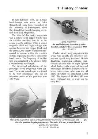
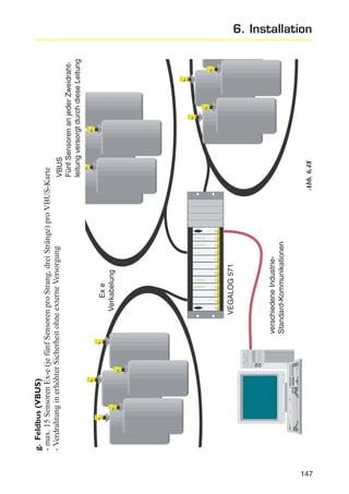
The original cavity magnetron had
a wavelength of 9.87 centimetres.
This corresponds to a frequency of
3037.4 MHz (3.0374 GHz).
The frequency of a pulse radar
level transmitter may be 26 GHz
or 26 x 108 metres per second.
The wavelength is 1.15 centimetres.
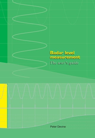
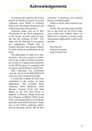
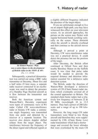
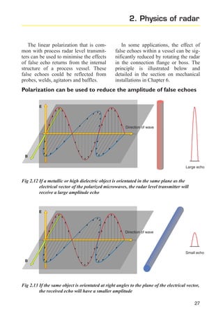
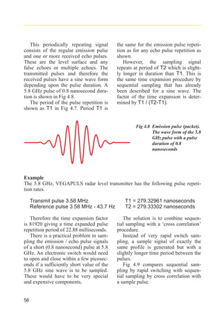
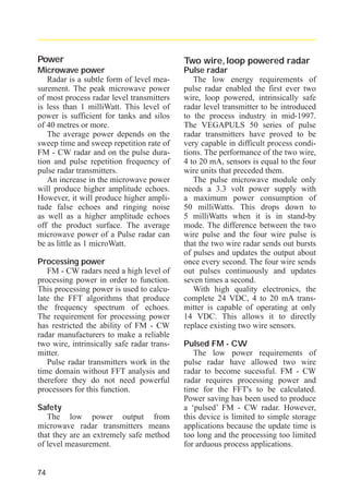
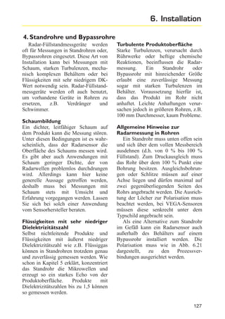
The electromagnetic waves have an
electrical vector E and a magnetic vector B that are perpendicular to each
other and perpendicular to the direction
of the wave. This will be discussed and
illustrated further in the section on
polarization. The electrical vector has
the major influence on radar applications.
λ
direction of wave
amplitude
co
(µ
The velocity of an electromagnetic
wave is the product of the frequency
and the wavelength.
Fig 2.1
13

20. The Electromagnetic spectrum
10 8
10 7
10 6
10 5
10 4
10 3
10 2
electric waves
10 1
10 2
10 1
10 0
10 -1
10 -2
10 -3 10 -4
radio waves
10 3
10 4
10 5
10 6
10 7
10 8
infra
10 9
10 10
10 11
10 12
3m
0.3 m
3 cm
3 mm
100 MHz
1 GHz
10 GHz
100 GHz
The microwave frequencies of the electromagnetic spectrum.
Radar level transmitters range between 5.8 GHz (5.2cm) and 26 GHz (11.5mm)
14

21. 2. Physics of radar
10 -5
10 -6
red
10 13
10 -7
10 -8
ultra violet
10 14
10 15
10 16
10 -9
10 -10 10 -11 10 -12 10 -13 10 -14 10 -15 10 -16
X rays
10 17
10 18
m
gamma rays
10 19
10 20
10 21
10 22
10 23
10 24
Hz
Fig 2.2 Electromagnetic spectrum.
All electromagnetic waves travel at the speed of light in free space. This spectrum
shows the range of frequencies and wavelengths from electric waves to
gamma rays
15

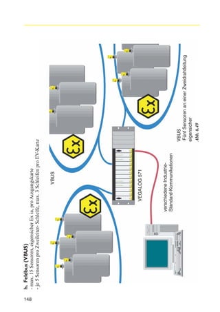
22. Permittivity
In electrostatics, the force between
two charges depends upon the magnitude and separation of the charges and
the composition of the medium
between the charges. Permittivity ε is
the property of the medium that effects
the magnitude of the force. The higher
the value of the permittivity, the lower
the force between the charges. The
value of the permittivity of free
space (in a vacuum) εo, is calculated
indirectly and empirically to be:
8.854 x 10-12 farad / metre.
Relative permittivity or
dielectric constant εr
The ratio of the permittivity of a
medium to the permittivity of free
space is a dimensionless property
called ‘relative permittivity’ or ‘dielectric constant’. For example, at 20° C
the relative permittivity of air is close
to that of a vaccum and is only about
1.0005 whereas the relative permittivity of water at 20° C is about 80.
(Dielectric constant is also widely
known as DK.)
The value of the dielectric constant
of the product being measured is very
important in the application of radar to
level measurement. In non-conductive
products, some of the microwave energy will pass through the product and
the rest will be reflected off the surface.
This feature of microwaves can be
used to advantage or, in some circumstances, it can create a measurement
problem.
16
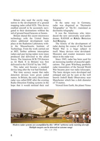
Permeability µ and relative
permeability µr
The magnetic vector, B, of an electromagnetic wave also has an influence
on the velocity of electromagnetic
waves. However, this influence is negligible when considering the velocity in
gases and vapours which are non-magnetic. The relative permeability of the
product being measured has no significant effect on the reflected signal when
compared with the effects of the relative permittivity or dielectric constant.
For the non-magnetic gases above the
product being measured, the value of
the relative permeability, µr = 1.
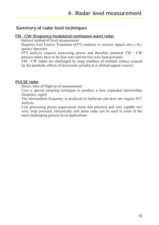
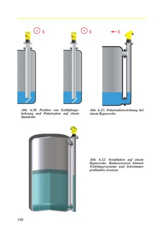
Frequency, velocity and wavelength
As we have already stated, the frequency (f), velocity (c) and wavelength
(λ) of the electromagnetic waves are
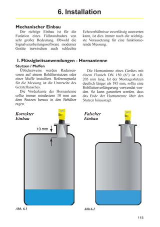
related by the equation c = f x λ.
The frequency remains uninfluenced
by changes in the propagation medium.
However, the velocity and wavelength
can change depending on the electrical
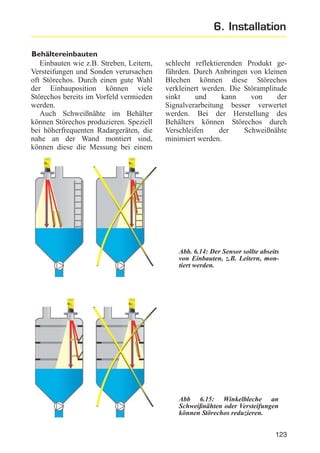
properties of the medium in which they
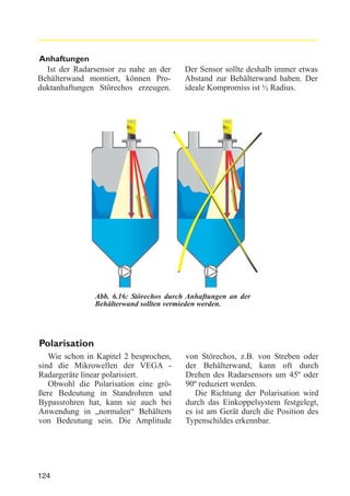
are travelling. The speed of propagation can be calculated using equation
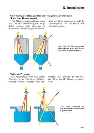
2.3.
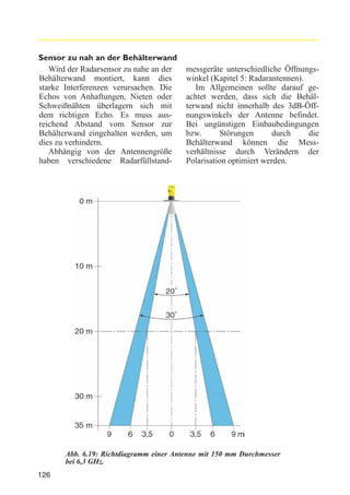
c =
co
(µ x ε )
r
c
co
µr
εr
r
[Eq. 2.3]
velocity of electromagnetic wave
in the medium in metres/second
velocity of electromagnetic
waves in free space
the relative permeability
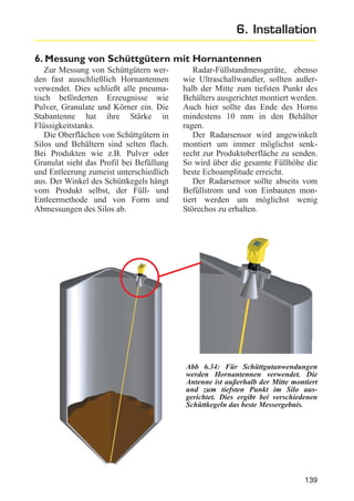
(µ medium / µo)
the relative permittivity

23. 2. Physics of radar
Changes in the wavelength and
velocity of microwaves are apparent in
certain radar level applications.
Changes in temperature, pressure and
gas composition have a small effect on
the running time of microwaves
because the dielectric constant of the
propagation medium is altered to a
greater or lesser extent. This is discussed in detail later.
Radar level transmitters can be used
to measure conductive liquids through
low dielectric ‘windows’ such as glass,
polypropylene and PTFE. The optimum thickness of the low dielectric
window is a half wavelength or multiple of half wavelength.
For example, polypropylene has a
dielectric constant εr of 2.3 and the
half wavelength at a frequency of 5.8
GHz is 17 mm compared with a half
wavelength of about 26 mm in a vacuum. It follows that the speed of
Empty vessel: large echo
from metal
bottom
microwaves in polypropylene is about
two thirds of the speed in air.
As with low dielectric windows,
non-conductive, low dielectric constant
liquids may absorb more power than
they reflect from the surface. The
velocity of the microwaves within the
liquid is slower than in the vapour
space above.
For example, if there is about 0.5
metres of solvent in the bottom of a
metallic vessel, a radar level transmitter
may see a larger echo from the vessel
bottom than from the product. This
large echo will appear to be further
away than it really is because the running time within the solvent is slower.
For this reason, special considerations
must be made within the echo processing software to ensure that the radar
follows the solvent level and does not
follow the vessel bottom as it apparently moves away!
As the vessel fills with
solvent two echoes
are received. The
echo from the vessel
bottom appears
further away because
the running time of
the microwaves in
solvent is slower
solvent echo
Fig 2.3 - Effect of dielectric constant on the running time of a microwave radar
17

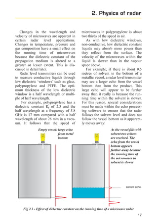
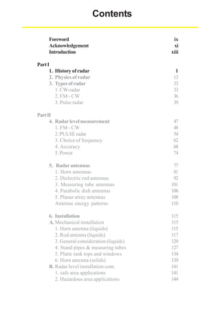
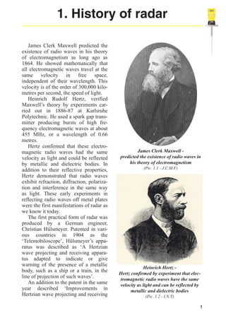
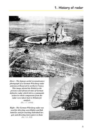
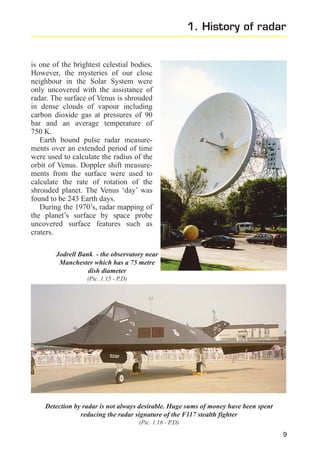
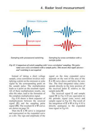
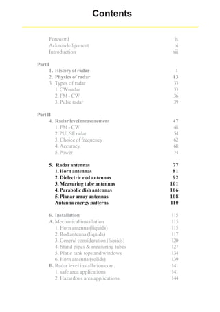
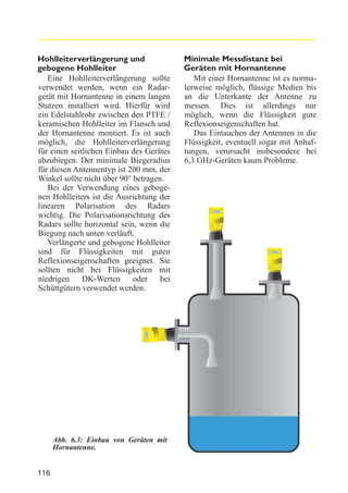
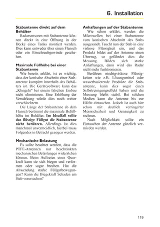
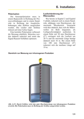
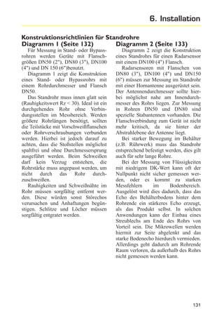
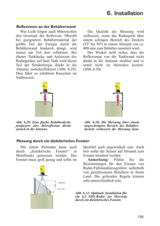
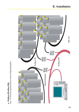
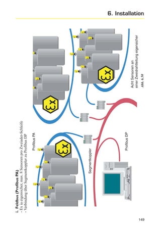
24. The same effect can be experienced when looking at interface detection using
guided microwave level transmitters to detect oil and water or solvent and aqueous
based liquids.
Fig 2.4 Oil/water interface
detection using a
guided microwave
level transmitter. Note
that the water echo
has a reduced amplitude and appears to be
further away. The
running time of
microwaves in oil is
slower than in air
reference echo
(water without oil)
oil echo
water echo
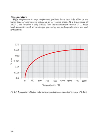
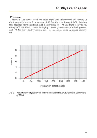
Effects on the propagation
speed of microwaves
Microwave radar level transmitters
can be applied almost universally
because, as a measurement technique,
they are virtually unaffected by process
temperature, temperature gradient, vacuum and normal pressure variations,
gas or vapour composition and movement of the propagation medium.
However, changes in these process
conditions do cause slight variations in
the propagation speed because the
dielectric constant of the propagation
medium is altered.
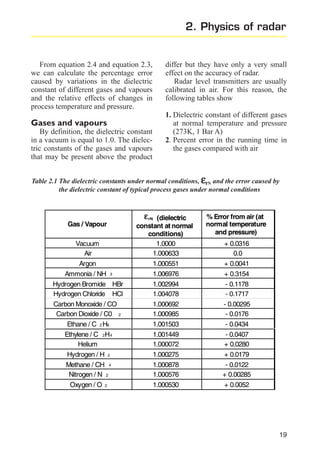
Calculating the propagation
speed of microwaves
The temperature, pressure and the
gas composition of the vapour space all
have an effect on the dielectric constant
of the propagation medium through
which the microwaves must travel.
This in turn affects the propagation
speed or running time of the instrument.
18
The dielectric constant or relative
permittivity can be calculated as
follows :
εr = 1 + (εrN - 1) x θN x P
θ x PN
[Eq. 2.4]
εr
εrN
calculated dielectric constant
(relative permittivity)
dielectric constant of gas/vapour
under normal conditions
(temperature 273 K, pressure 1 bar
absolute)
θN
PN
θ
P
temperature under normal
conditions, 273 Kelvin
pressure under normal
conditions, 1 bar absolute
process temperature in Kelvin
process pressure in bar absolute

25. 2. Physics of radar
From equation 2.4 and equation 2.3,
we can calculate the percentage error
caused by variations in the dielectric
constant of different gases and vapours
and the relative effects of changes in
process temperature and pressure.
Gases and vapours
By definition, the dielectric constant
in a vacuum is equal to 1.0. The dielectric constants of the gases and vapours
that may be present above the product
differ but they have only a very small
effect on the accuracy of radar.
Radar level transmitters are usually
calibrated in air. For this reason, the
following tables show
1. Dielectric constant of different gases
at normal temperature and pressure
(273K, 1 Bar A)
2. Percent error in the running time in
the gases compared with air
Table 2.1 The dielectric constants under normal conditions, εrN and the error caused by
the dielectric constant of typical process gases under normal conditions
% Error from air (at
normal temperature
and pressure)
Vacuum
Air
Argon
Ammonia / NH 3
Hydrogen Bromide HBr
Hydrogen Chloride HCl
Carbon Monoxide / CO
Carbon Dioxide / C0 2
Ethane / C 2 H6
Ethylene / C 2H4
Helium
ε rN (dielectric
constant at normal
conditions)
1.0000
1.000633
1.000551
1.006976
1.002994
1.004078
1.000692
1.000985
1.001503
1.001449
1.000072
Hydrogen / H 2
Methane / CH 4
Nitrogen / N 2
Oxygen / O 2
1.000275
1.000878
1.000576
1.000530
+ 0.0179
- 0.0122
+ 0.00285
+ 0.0052
Gas / Vapour
+ 0.0316
0.0
+ 0.0041
+ 0.3154
- 0.1178
- 0.1717
- 0.00295
- 0.0176
- 0.0434
- 0.0407
+ 0.0280
19

26. Temperature
High temperature or large temperature gradients have very little effect on the
transit time of microwaves within an air or vapour space. At a temperature of
2000° C the variation is only 0.026% from the measurement value at 0° C. Radar
level transmitters with air or nitrogen gas cooling are used on molten iron and steel
applications.
0.03
0.025
% error
0.02
0.015
0.01
0.005
0.0
0
250
500
750
1000
1250
1500
1750
2000
Temperature in ° C
Fig 2.5 Temperature effect on radar measurement of air at a constant pressure of 1 BarA
20

27. 2. Physics of radar
Pressure
Pressure does have a small but more significant influence on the velocity of
electromagnetic waves. At a pressure of 30 Bar, the error is only 0.84%. However
this becomes more significant and at a pressure of 100 Bar there is a velocity
change of 2.8%. If the pressure is varying constantly between atmospheric pressure
and 100 Bar, the velocity variations can be compensated using a pressure transmitter.
10
% error
8
6
4
2
0
0
50
100
150
200
250
300
350
400
Pressure in Bar (absolute)
Fig 2.6 The influence of pressure on radar measurement in air at a constant temperature
of 273 K
21

28. Waveguides, stilling tubes & bypass tubes
In the preceding equations, we have
assumed that the microwaves are
travelling in ‘free space’ in a vacuum.
However, in practice the proximity
of metallic vessel walls and other
structures will have an influence on
the propagation velocity of the
microwaves. This is particularly true
when microwave radar level transmitters are fitted inside bypass tubes or
stilling tubes or when a horn antenna is
fitted with a waveguide extension.
When microwaves are propagating
within a metallic tube the running time
appears to slow down because the
microwaves travel further bouncing
off the inside wall of the tube and
currents are set up on the inside surface
of the tube.
This effect is discussed in more
detail in the chapters on antennas and
mechanical installations. The waveguide effect can be compensated during
calibration and the use of stilling tubes
and bypass tubes can be beneficial in
some level applications.
Electromagnetic waves exhibit the same properties as light.
·
·
·
Reflection
Polarization
Diffraction
·
·
Refraction
Interference
Reflection of electromagnetic waves
Conductive products
Using a spark gap transmitter,
Heinrich Hertz demonstrated that electromagnetic waves could be reflected
off metallic objects and objects with a
relatively high dielectric constant.
In the same way, radar can easily
measure conductive aqueous liquids
such as acids and caustic and other
conductive products ranging from
molten metal to saturated spent grain in
the brewing process.
When microwaves from a radar hit a
conductive surface the electrical field E
is short circuited. The resultant current
in the conductive product causes the
microwaves to be re-transmitted or
reflected from the surface.
22
Radar level transmitters have no
problem in measuring conductive liquids and solids because the microwaves
with frequencies between 5.8 GHz and
26GHz are readily reflected off a conductive surface producing relatively
large echoes.
Non-conductive products
If a liquid or solid is non-conductive,
the value of the dielectric constant (relative permittivity εr) becomes more
important. The theoretical amount of
reflection at a dielectric layer can be calculated using equation 2.5

29. 2. Physics of radar
W1
Transmitted power:
W2
Reflected power:
Dielectric constant:
εr
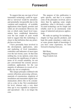
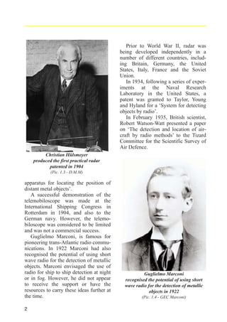
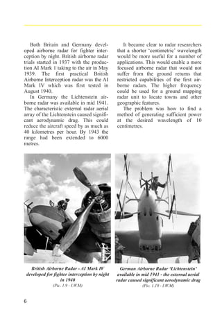
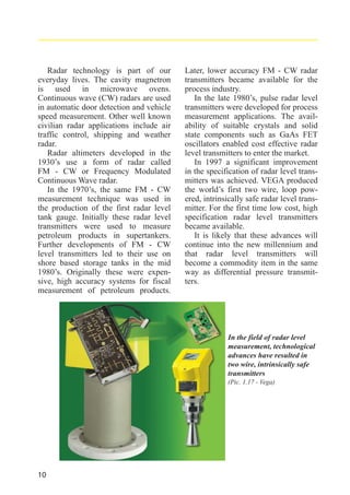
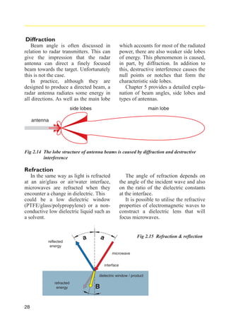
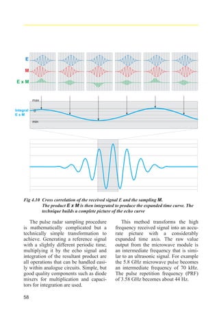
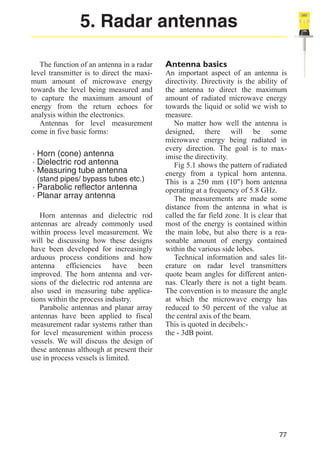
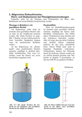
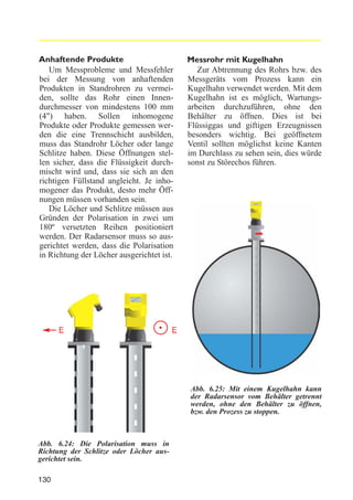
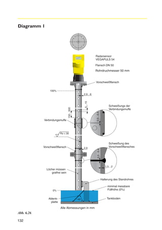
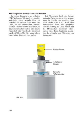
Then the percentage of reflected
power at the dielectric layer,
Π = 1-
4 x εr
(1 + ε )
2
r
W2
Π =
[Eq. 2.5]
W1
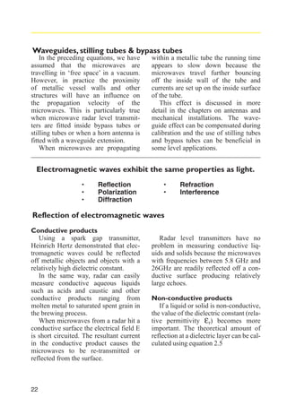
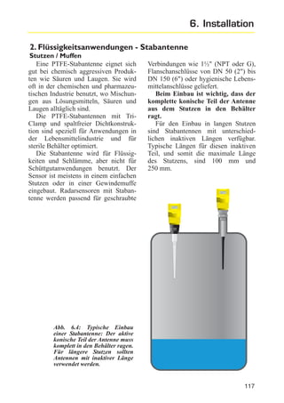
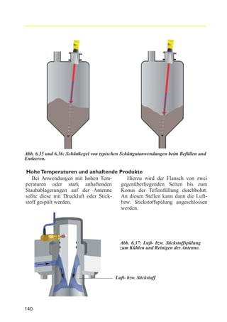
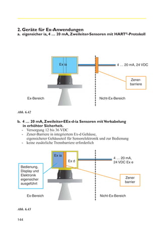
Typical examples are as follows:
Acetone
Solvent with a dielectric constant,
εr = 20
Toluene
Solvent with a low dielectric consta t
n,
εr = 2.4
Π = 1-
(2.4)
4x
(1 +
Π = 1-
2
(2.4))
4.46% power is reflected
4x
(1 +
( 20 )
(20)
2
)
40 % power is reflected
Π x 100% power reflected
100
80
60
40
20
0
0
10
20
30
40
50
60
70
80
Dielectric constant, εr
Fig 2.7 Reflected radar power depends upon the dielectric constant of the product
being measured
23

30. In radar level measurement the reflected energy from a product surface becomes
more critical at a dielectric constant (εr) of less than 5. The following graph shows
this important region.
Π x 100% power reflected
20
15
10
5
0
1.0
1.5
2.0
3.0
2.5
3.5
Dielectric constant, εr
4.0
4.5
5.0
Fig 2.8 Reflected radar power depends upon the dielectric constant of the product being
measured. This graph shows the critical region where care must be taken over
choice of radar antenna
0
Loss L, dB
- 10
- 20
- 40
- 60
3.0
3.5
2.5
Dielectric constant, εr
Fig 2.9 Reflection loss in dB: loss L = 10 log Π
1.0
1.5
2.0
4.0
4.5
5.0
Most electrically conductive products or products with a dielectric constant of
more than 1.5 can be measured using microwave radar level transmitters. Stilling
tubes can be used to concentrate the microwaves for lower dielectric constant
products.
24

31. 2. Physics of radar
Polarization
Electromagnetic waves have an
electrical vector E and magnetic vector
B that are in phase but perpendicular to
each other. The direction of propagation of the waves is perpendicular to
the electrical and magnetic vectors as
shown in the diagram below.
Polarization defines the orientation
of the electromagnetic waves and refers
to the direction of the electrical vector
E. Most process radar level transmitters
exhibit linear polarization as in the dia-
gram. The direction of the linear polarization is set by the orientation of the
signal coupler from the microwave
module. The properties of the polarization of microwaves can be important in
the application of radar to level measurement.
In television and microwave communications, linear polarization is also
referred to as horizontal or vertical
polarization depending on the relative
orientation of the aerials or antennas.
E
direction of wave
B
Fig 2.10 Diagram showing linear polarization and the relative orientation of the electric
vector E, the magnetic vector B and the direction of propagation of the
microwaves
25

32. Another form of polarization is
elliptical polarization. A specific form
of elliptical polarization is circular
polarization where the electrical vector
E and magnetic vector B rotate through
360° within the space of a single wavelength, when a linear or circular polarized signal is reflected the direction of
polarization is reversed. With circular
polarization it is possible to use the
reversal of polarization to distinguish
between a direct echo and an echo that
has made two reflections.
Circular polarization can also be
used in search radars to separate the
reflections from aircraft or ships from
interference echoes from rain. The
almost spherical shape of the rain drops
causes a definite reversal of polarization which can be easily rejected by the
receiving antenna. However, the scattered reflections from the ship or aircraft provide roughly equal amounts of
reversed and un-reversed energy that
enables detection.
λ
Fig 2.11 Circular polarization involves rotation of the electrical and magnetic vectors
through 360° within a wavelength
26

33. 2. Physics of radar
The linear polarization that is common with process radar level transmitters can be used to minimise the effects
of false echo returns from the internal
structure of a process vessel. These
false echoes could be reflected from
probes, welds, agitators and baffles.
In some applications, the effect of
false echoes within a vessel can be significantly reduced by rotating the radar
in the connection flange or boss. The
principle is illustrated below and
detailed in the section on mechanical
installations in Chapter 6.
Polarization can be used to reduce the amplitude of false echoes
E
Direction of wave
B
Large echo
Fig 2.12 If a metallic or high dielectric object is orientated in the same plane as the
electrical vector of the polarized microwaves, the radar level transmitter will
receive a large amplitude echo
E
Direction of wave
Small echo
B
Fig 2.13 If the same object is orientated at right angles to the plane of the electrical vector,
the received echo will have a smaller amplitude
27

34. Diffraction
Beam angle is often discussed in
relation to radar transmitters. This can
give the impression that the radar
antenna can direct a finely focused
beam towards the target. Unfortunately
this is not the case.
In practice, although they are
designed to produce a directed beam, a
radar antenna radiates some energy in
all directions. As well as the main lobe
which accounts for most of the radiated
power, there are also weaker side lobes
of energy. This phenomenon is caused,
in part, by diffraction. In addition to
this, destructive interference causes the
null points or notches that form the
characteristic side lobes.
Chapter 5 provides a detailed explanation of beam angles, side lobes and
types of antennas.
side lobes
main lobe
antenna
Fig 2.14 The lobe structure of antenna beams is caused by diffraction and destructive
interference
Refraction
In the same way as light is refracted
at an air/glass or air/water interface,
microwaves are refracted when they
encounter a change in dielectric. This
could be a low dielectric window
(PTFE/glass/polypropylene) or a nonconductive low dielectric liquid such as
a solvent.
reflected
energy
The angle of refraction depends on
the angle of the incident wave and also
on the ratio of the dielectric constants
at the interface.
It is possible to utilise the refractive
properties of electromagnetic waves to
construct a dielectric lens that will
focus microwaves.
a
a
Fig 2.15 Refraction & reflection
microwave
interface
dielectric window / product
refracted
energy
28
B

35. 2. Physics of radar
Interference - Phase
Problematic interference effects are caused primarily by the inadvertent mixing
of signals that are out of phase. The microwave signals have a sinusoidal waveform.
Phase angle
45°
Fig 2.16 In this illustration both of the sine waves have an identical frequency and
amplitude but the second wave has a 45° phase lag
Interference can be ‘constructive’ where in-phase signals produce a signal with a
higher amplitude or it can be destructive where signals that are 180° out of phase
effectively cancel each other out.
signals in-phase
constructive interference
180° out of phase
destructive interference
Fig 2.17 Illustration of constructive and destructive interference
29

36. Interference
Microwaves can manifest interference effects in exactly the same way as
light. Potentially this can cause measurement problems. The causes of
interference should be understood and
avoided by design and installation considerations.
The wrong choice of antenna, installation of an antenna up a nozzle, positioning transmitters too close to vessel
walls or other obstructions can all lead
to interference of the signal. The chapter on mechanical installation should
help a radar level user to avoid this
potential problem.
However, we use destructive interference to our advantage when we
apply pulse radar level measurement
through a low dielectric ‘window’ to
measure conductive or high dielectric
liquids.
A
+
=
C
B’
B
B”
Fig 2.18 Interference caused by positioning an antenna too close to the vessel wall. If a
radar level transmitter is installed too close to the vessel wall it is possible that
interference will occur. With indirect reflection A B’ B’’ C, the phase may be
altered by 180° when compared with the direct reflection A B C. For this reason
the microwaves may partially cancel out due to destructive interference
30

37. 2. Physics of radar
The thickness of the dielectric window must be a half wavelength of the
window material. When the half wavelength is used, there is destructive interference between the reflection off the
top surface of the window and the
reflection off the internal second surface
of the window.
There is a 180° phase shift between
these reflections and they cancel each
emitted wave
plastic vessel ceiling
other out. This type of installation
is explained more fully in Chapter 6
on the mechanical installations of
radar level transmitters together with
a table showing the optimum thickness
of most important plastics and glasses
which are suitable for penetration with
radar sensors.
reflection with
phase shift from top
surface
reflection without
phase shift from
internal surface
D
emitted wave
reflection with phase shift off
top surface of window
reflection without phase shift
off internal face of window
Fig 2.19 Destructive interference is a benefit when using pulse radar to measure through
a low dielectric window. The reflection from the top surface and the reflection
from the internal second surface cancel each other if the thickness is a half
wavelength
31

38. Contents
Foreword
Acknowledgement
Introduction
ix
xi
xiii
Part I
1. History of radar
2. Physics of radar
3. Types of radar
1. CW-radar
2. FM - CW
3. Pulse radar
1
13
33
33
36
39
Part II
4. Radar level measurement
1. FM - CW
2. PULSE radar
3. Choice of frequency
4. Accuracy
5. Power
47
48
54
62
68
74
5. Radar antennas
1. Horn antennas
2. Dielectric rod antennas
3. Measuring tube antennas
4. Parabolic dish antennas
5. Planar array antennas
Antenna energy patterns
77
81
92
101
106
108
110
6. Installation
A. Mechanical installation
1. Horn antenna (liquids)
2. Rod antenna (liquids)
3. General consideration (liquids)
4. Stand pipes & measuring tubes
5. Platic tank tops and windows
6. Horn antenna (solids)
B. Radar level installation cont.
1. safe area applications
2. Hazardous area applications
115
115
115
117
120
127
134
139
141
141
144

39. 3. Types of radar
1a. CW, continuous wave radar
In continuous wave or CW Radar, a
continuous unmodulated frequency is
transmitted and echoes are received
from the target object. If the target
object is stationary, the frequency of
the return echoes will be the same as
the transmitted frequency. The range of
the object cannot be measured.
However, the frequency of the return
signal from a moving object is changed
depending on the speed and direction
of the object. This is the well known
‘doppler effect’. The doppler effect is
apparent when the siren note of an
emergency vehicle changes as it speeds
past a pedestrian. The pitch of the siren
note is higher as it approaches the listener and lower as it recedes. The
doppler effect is also used by
astronomers to monitor the expansion
of the Universe. By measuring the ‘red
shift’ of the spectrum of distant stars
and galaxies the rate of expansion can
be measured and the age of distant
objects can be estimated.
In the same way, when an object that
has been illuminated by a CW Radar
approaches the transmitter, the frequency of the return signal will be higher
than the transmitted frequency. The
echo frequency will be lower if the
object is moving away.
yv
elocit
rece
requ
ived f
tv
targe
f + f dp
ency t
itted
m
trans
ave
yf w
uenc t,
lengt
hλ
freq
Fig 3.1 CW radar uses doppler shift to derive speed measurement
33

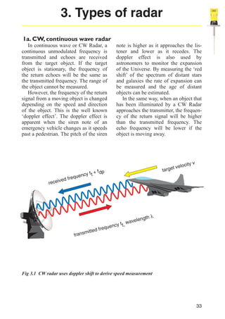
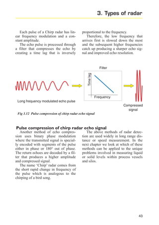
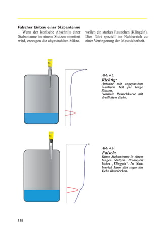
40. In Fig 3.1, the aircraft is travelling
towards the CW radar. Therefore the
received frequency is higher than
the transmitted frequency and the sign
of fdp is positive. If the aircraft was
travelling away from the radar at the
v =
λ x fdp
2
=
same speed, the received frequency
would be ft - fdp.
The velocity of the target in the
direction of the radar is calculated by
equation 3.1
c x fdp
c
v
ft
2 x ft
fdp
[Eq. 3.1]
ft+fdp
is the velocity of microwaves
is the target velocity
is the frequency of the
transmitted signal
is the doppler beat frequency
which is proportional to velocity
is received frequency. The sign
of fdp depends upon whether the
target is closing or receding
1b. CW wave-interference radar or bistatic CW radar
We have already mentioned that CW
radar was used in early radar detection
experiments such as the famous
Daventry experiment carried out by
Robert Watson - Watt and his colleagues. In this case, the transmitter
and receiver were separated by a considerable distance. A moving object
was detected by the receiver because
there was interference between the fre-
quency received directly from the
transmitter and the doppler shifted frequency reflected off the target object.
Although the presence of the object is
detected, the position and speed cannot
be calculated.
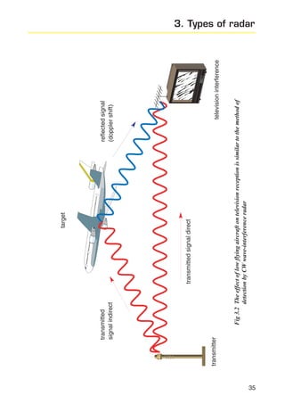
In essence, this is what happens
when a low flying aircraft interferes
with the picture on a television screen.
See Fig 3.2.
1c. Multiple frequency CW radar
Standard continuous wave radar is
used for speed measurement and, as
already explained, the distance to a stationary object can not be calculated.
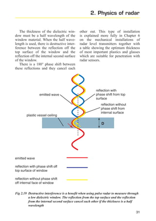
However, there will be a phase shift
between the transmitted signal and the
return signal.
If the starting position of the object
is known, CW radar could be used to
detect a change in position of up to half
wavelength (λ/2) of the transmitted
wave by measuring the phase shift of
the echo signal. Although further
movement could be detected, the range
34
would be ambiguous. With microwave
frequencies this means that the useful
measuring range would be very limited.
If the phase shifts of two slightly
different CW frequencies are measured
the unambiguous range is equal to the
half wavelength (λ/2) of the difference
frequency. This provides a usable distance measurement device.
However, this technique is limited to
measurement of a single target.
Applications include surveying and
automobile obstacle detection.

41. transmitter
transmitted signal direct
television interference
reflected signal
(doppler shift)
Fig 3.2 The effect of low flying aircraft on television reception is similar to the method of
detection by CW wave-interference radar
transmitted
signal indirect
target
3. Types of radar
35

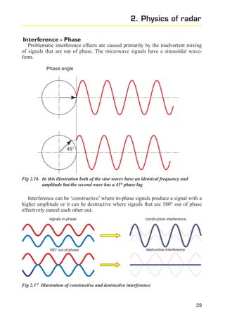
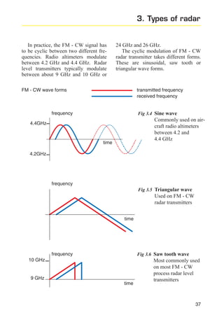
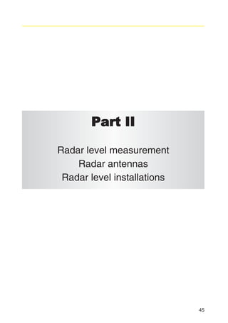
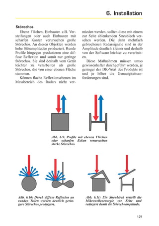
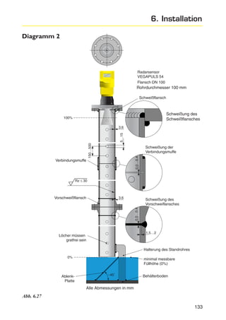
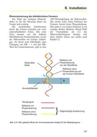
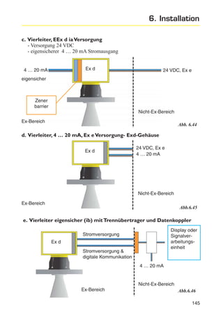
42. 2.
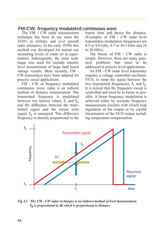
FM-CW, frequency modulated continuous wave radar
If the distance to the target is R,
and c is the speed of light, then the
time taken for the return journey is:-
2xR
c
∆t =
[Eq. 3.2]
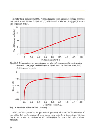
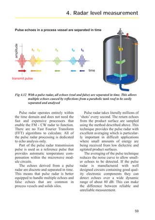
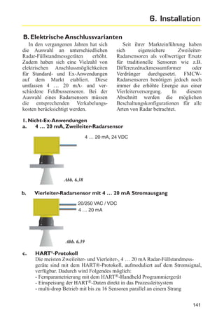
We can see from Fig. 3.3 that if
we know the linear rate of change of
the transmitted signal and measure the
difference between the transmitted and
received frequency fd, then we can
calculate the time ∆t and hence derive
the distance R.
frequency
Single frequency CW radar cannot
be used for distance measurement
because there is no time reference mark
to gauge the delay in the return echo
from the target. A time reference mark
can be achieved by modulating the frequency in a known manner.
If we consider the frequency of the
transmitted signal ramping up in a
linear fashion, the difference between
the transmitting frequency and the
frequency of the returned signal will be
proportional to the distance to the
target.
cy
en
u
eq
r
df
itte
m
ns
tra
re
∆t
fd
c
e
eiv
df
re
e
qu
nc
y
∆t =
2xR
c
time
Fig 3.3 The principle of FM - CW radar
36

43. 3. Types of radar
In practice, the FM - CW signal has
to be cyclic between two different frequencies. Radio altimeters modulate
between 4.2 GHz and 4.4 GHz. Radar
level transmitters typically modulate
between about 9 GHz and 10 GHz or
24 GHz and 26 GHz.
The cyclic modulation of FM - CW
radar transmitter takes different forms.
These are sinusoidal, saw tooth or
triangular wave forms.
FM - CW wave forms
transmitted frequency
received frequency
frequency
Fig 3.4 Sine wave
Commonly used on aircraft radio altimeters
between 4.2 and
4.4 GHz
4.4GHz
time
4.2GHz
frequency
Fig 3.5 Triangular wave
Used on FM - CW
radar transmitters
time
frequency
Fig 3.6 Saw tooth wave
10 GHz
9 GHz
time
Most commonly used
on most FM - CW
process radar level
transmitters
37

44. If we look at a triangular wave
form we can see that there is an interruption in the output of the difference
frequency , fd. In practice, the received
signal is heterodyned with part of the
transmitted frequency to produce the
difference frequency which has a posi-
tive value independent of whether the
modulation is increasing or decreasing.
The diagram below makes the
assumption that the target distance is
not changing. If the target is moving,
there will be a doppler shift in the difference frequency.
frequency
time
difference
frequency
fd
time
Fig 3.7 & 3.8 The change in direction between the ramping up and down of the frequency
creates a short break in the measured value of the difference frequency.
This has to be filtered out. The transmitted frequency is represented by the
red line and the received frequency is represented by the dark blue line.
The difference frequency is shown in light blue on the bottom graph
38

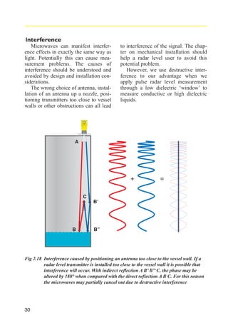
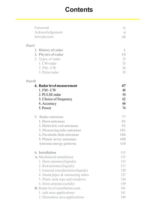
45. 3. Types of radar
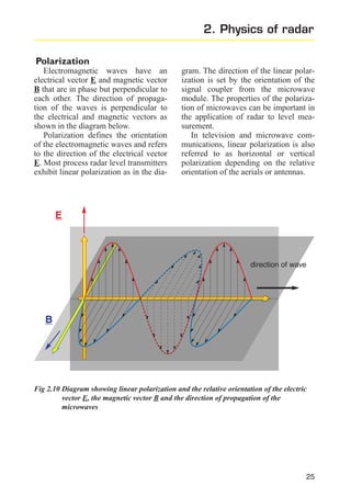
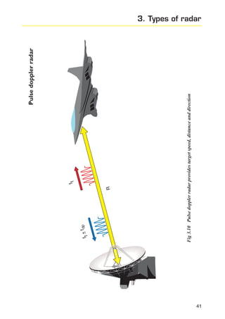
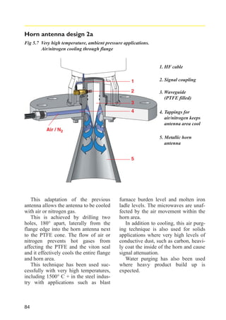
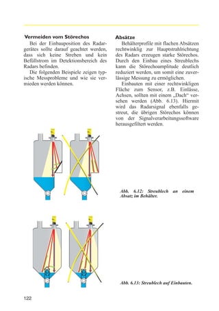
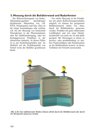
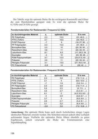
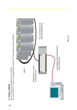
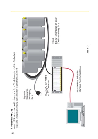
3. Pulse radar
a. Basic pulse radar
Pulse radar is and has been used
widely for distance measurement since
the very beginnings of radar technology. The basic form of pulse radar is a
pure time of flight measurement. Short
pulses, typically of millisecond or
nansecond duration, are transmitted
and the transit time to and from the target is measured.
The pulses of a pulse radar are not
discrete monopulses with a single peak
of electromagnetic energy, but are in
fact a short wave packet. The number
of waves and length of the pulse
depends upon the pulse duration and
the carrier frequency that is used.
These regularly repeating pulses
have a relatively long time delay
between them to allow the return echo
to be received before the next pulse is
transmitted.
t
τ
3rd pulse
2nd pulse
1st pulse
Transmitted pulses
Fig 3.9 Basic pulse radar
The inter pulse period (the time
between successive pulses) t is the
inverse of the pulse repetition
frequency fr or PRF. The pulse duration
or pulse width, τ, is a fraction of the
inter pulse period.
The inter pulse period t effectively
defines the maximum range of the
radar.
Example
The pulse repetition frequency
(PRF) is defined as
fr =
1
t
If the pulse period t is 500 microseconds, then the pulse repetition frequency is two thousand pulses per second.
In 500 microseconds, the radar pulses
will travel 150 kilometres. Considering
the return journey of an echo reflected
off a target, this gives a maximum theoretical range of 75 kilometres.
If the time taken for the return
journey is T, and c is the speed of light,
then the distance to the target is
R=
Txc
2
[Eq. 3.3]
39

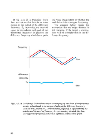
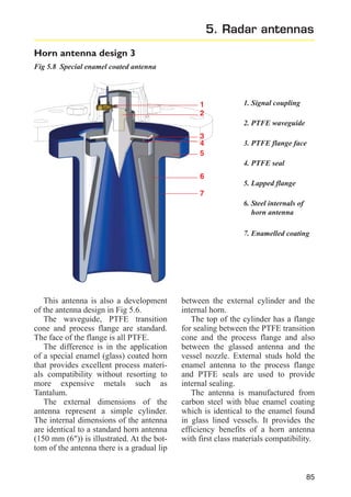
46. b. Pulse doppler radar
The pulses transmitted by a standard
pulse radar can be considered as a very
short burst of continuous wave radar.
There is a single frequency with no
modulation on the signal for the duration of the pulse.
If the frequency of the waves of the
transmitted pulse is ft and the target is
moving towards the radar with velocity
v, then, as with the CW radar already
described, the frequency of the return
pulse will be ft + fdp , where fdp is the
doppler beat frequency. Similarly, the
received frequency will be ft - fdp if the
target is moving away from the radar.
Therefore, a pulse doppler radar can
be used to measure speed, distance and
direction.
The ability of the pulse doppler
radar to measure speed allows the system to ignore stationary targets. This is
also commonly called ‘moving target
indication’ or MTI radar.
In general, an MTI radar has accurate range measurement but imprecise
speed measurement, whereas a pulse
doppler radar has accurate speed measurement and imprecise distance measurement.
40
The velocity of the target in the
direction of the radar is calculated in
equation 3.4:
c =
c x fdp
λ x fdp
=
2 x ft
2
[Eq. 3.4]
This is the same calculation as for
CW radar. The distance to the target is
calculated by the transit time of the
pulse, equation 3.3.
R =
Txc
2
[Eq. 3.3]
As well as being used to monitor
civil and military aircraft movements,
pulse doppler radar is used in weather
forecasting. A doppler shift is measured
within storm clouds which can be distinguished from general ground clutter. It is also used to measure the
extreme wind velocities within a tornado or ‘twister’.

47. R
Fig 3.10 Pulse doppler radar provides target speed, distance and direction
f t + f dp
ft
Pulse doppler radar
3. Types of radar
41

48. c. Pulse compression and ‘Chirp’ radar
frequency
With pulse radar, a shorter pulse
duration enables better target resolution
and
therefore
higher
accuracy.
However, a shorter pulse needs a significantly higher peak power if the
range performance has to be maintained. If there is a limit to the maximum power available, a short pulse
will inevitably result in a reduced
range.
With limited peak power, a longer
pulse duration, τ , will provide more
radiated energy and therefore range but
(with a standard pulse radar) at the
expense of resolution and accuracy.
Pulse compression within a ‘Chirp’
radar is a method of achieving the
accuracy benefits of a short pulse radar
together with the power benefits of
using a longer pulse. Essentially, Chirp
radar is a cross between a pulse radar
and an FM - CW radar.
f1
f2
time
t2
t1
amplitude
τ
time
Fig 3.11 Chirp radar wave form. Chirp is a cross between pulse and FM - CW radar
42

49. 3. Types of radar
Each pulse of a Chirp radar has linear frequency modulation and a constant amplitude.
The echo pulse is processed through
a filter that compresses the echo by
creating a time lag that is inversely
proportional to the frequency.
Therefore, the low frequency that
arrives first is slowed down the most
and the subsequent higher frequencies
catch up producing a sharper echo signal and improved echo resolution.
Time lag
Filter
Frequency
Long frequency modulated echo pulse
Compressed
signal
Fig 3.12 Pulse compression of chirp radar echo signal
Pulse compression of chirp radar echo signal
Another method of echo compression uses binary phase modulation
where the transmitted signal is specially encoded with segments of the pulse
either in phase or 180° out of phase.
The return echoes are decoded by a filter that produces a higher amplitude
and compressed signal.
The name ‘Chirp’ radar comes from
the short rapid change in frequency of
the pulse which is analogous to the
chirping of a bird song.
The above methods of radar detection are used widely in long range distance or speed measurement. In the
next chapter we look at which of these
methods can be applied to the unique
problems involved in measuring liquid
or solid levels within process vessels
and silos.
43

50. Part II
Radar level measurement
Radar antennas
Radar level installations
45

51. Contents
Foreword
Acknowledgement
Introduction
ix
xi
xiii
Part I
1. History of radar
2. Physics of radar
3. Types of radar
1. CW-radar
2. FM - CW
3. Pulse radar
1
13
33
33
36
39
Part II
4. Radar level measurement
1. FM - CW
2. PULSE radar
3. Choice of frequency
4. Accuracy
5. Power
47
48
54
62
68
74
5. Radar antennas
1. Horn antennas
2. Dielectric rod antennas
3. Measuring tube antennas
4. Parabolic dish antennas
5. Planar array antennas
Antenna energy patterns
77
81
92
101
106
108
110
6. Installation
A. Mechanical installation
1. Horn antenna (liquids)
2. Rod antenna (liquids)
3. General consideration (liquids)
4. Stand pipes & measuring tubes
5. Platic tank tops and windows
6. Horn antenna (solids)
B. Radar level installation cont.
1. safe area applications
2. Hazardous area applications
115
115
115
117
120
127
134
139
141
141
144

52. radar_applied_to_level_rb.qxd
15.01.2007
18:46
Seite 47
4. Radar level measurement
The benefits of radar as a level measurement technique are clear.
Radar provides a non-contact sensor
that is virtually unaffected by changes
in process temperature, pressure or the
gas and vapour composition within a
vessel.
In addition, the measurement accuracy is unaffected by changes in density, conductivity and dielectric constant
of the product being measured or by air
movement above the product.
The practical use of microwave
radar for tank gauging and process vessel level measurement introduces an
interesting set of technical challenges
that have to be mastered.
If we consider that the speed of light
is approximately 300,000 kilometres
per second. Then the time taken for
a radar signal to travel one metre
and back takes 6.7 nanoseconds or
0.000 000 006 7 seconds.
How is it possible to measure this
transit time and produce accurate vessel contents information?
Currently there are two measurement techniques in common use for
process vessel contents measurement.
They are frequency modulated continuous wave (FM - CW) radar and PULSE
radar
In this chapter we explain FM - CW
and PULSE radar level measurement
and compare the two techniques. We
discuss accuracy and frequency considerations and explore the technical
advances that have taken place in
recent years and in particular two wire,
loop powered transmitters.
47

53. radar_applied_to_level_rb.qxd
15.01.2007
18:46
Seite 48
FM-CW, frequency modulated continuous wave
The FM - CW radar measurement
technique has been in use since the
1930's in military and civil aircraft
radio altimeters. In the early 1970's this
method was developed for marine use
measuring levels of crude oil in supertankers. Subsequently, the same technique was used for custody transfer
level measurement of large land based
storage vessels. More recently, FM CW transmitters have been adapted for
process vessel applications.
FM - CW, or frequency modulated
continuous wave, radar is an indirect
method of distance measurement. The
transmitted frequency is modulated
between two known values, f1 and f2,
and the difference between the transmitted signal and the return echo
signal, fd, is measured. This difference
frequency is directly proportional to the
transit time and hence the distance.
(Examples of FM - CW radar level
transmitters modulation frequencies are
8.5 to 9.9 GHz, 9.7 to 10.3 GHz and 24
to 26 GHz).
The theory of FM - CW radar is
simple. However, there are many practical problems that need to be
addressed in process level applications.
An FM - CW radar level transmitter
requires a voltage controlled oscillator,
VCO, to ramp the signal between the
two transmitted frequencies, f1 and f2.
It is critical that the frequency sweep is
controlled and must be as linear as possible. A linear frequency modulation is
achieved either by accurate frequency
measurement circuitry with closed loop
regulation of the output or by careful
linearisation of the VCO output including temperature compensation.
f2
frequency
Transmitted signal
fd
∆t
Received
signal
f1
t1
time
Fig 4.1 The FM - CW radar technique is an indirect method of level measurement.
fd is proportional to ∆t which is proportional to distance
48

54. f(t)
Directional
Coupler
Signal sampling
and
Fast Fourier transforms (FFT)
Frequency
Measurement
Intermediate
frequency
Amplifier
Filter
Mixer
f (t + Dt)
Directional
Coupler
f (t + Dt)
Fig 4.2 Typical block diagram of FM - CW radar. A very accurate linear sweep is required
Signal Microprocessor
Front end control function
Linear ramp generator
Voltage
Control
V(t)
Linear sweep
control loop
Voltage Controlled Oscillator VCO
f(t)
4. Radar level measurement
49

55. radar_applied_to_level_rb.qxd
15.01.2007
FM - CW block diagram (Fig 4.2)
The essential component of a frequency modulated continuous wave
radar is the linear sweep control circuitry. A linear ramp generator feeds a
voltage controller which in turn ramps
up the frequency of the Voltage
Controlled Oscillator. A very accurate
linear sweep is required. The output
frequency is measured as part of the
closed loop control.
The frequency modulated signal is
directed to the radar antenna and
18:46
Seite 50
hence towards the product in the vessel. The received echo frequencies are
mixed with a part of the transmission
frequency signal. These difference frequencies are filtered and amplified
before Fast Fourier Transform (FFT)
analysis is carried out. The FFT
analysis produces a frequency spectrum on which the echo processing and
echo decisions are made.
Pic 2 Typical glass lined
agitated process
vessel. A radar
must be able to
cope with various
false echos from
agitatior blades
and baffles
Simple storage applications usually
have a large surface area with very little agitation, no significant false echoes
from the internal structure of the tank
and relatively slow product movement.
These are the ideal conditions for
which FM - CW radar was originally
developed.
However, in process vessels there is
more going on and the problems
become more challenging.
50
Low amplitude signals and false
echoes are common in chemical reactors where there is agitation and low
dielectric liquids.
Solids applications can be troublesome because of the internal structure
of the silos and undulating product surfaces which creates multiple echoes.
An FM - CW radar level sensor
transmits and receives signals simultaneously.

56. radar_applied_to_level_rb.qxd
15.01.2007
18:46
Seite 51
4. Radar level measurement
fd1, -f d2 , -fd3, -fd4, -fd5
f2
f1
t1
Transmitted signal
Real echo signal
False echo signals
Fig 4.3a FM - CW radar level transmitters in an active process vessel
In an active process vessel, the various echoes are received as frequency
differences compared with the frequency of the transmitting signal. These frequency difference signals are received
by the antenna at the same time. The
amplitude of the real echo signals are
small compared with the transmitted
signal. A false echo from the end of the
antenna may have a significantly higher amplitude than the real level echo.
The system needs to separate and identify these simultaneous signals before
processing the echoes and making an
echo decision.
The separation of the various
received echo frequencies is achieved
using Fast Fourier Transform (FFT)
analysis. This is a mathematical proce-
dure which converts the jumbled array
of difference frequencies in the time
domain into a frequency spectrum in
the frequency domain.
The relative amplitude of each frequency component in the frequency
spectrum is proportional to the size of
the echo and the difference frequency
itself is proportional to the distance
from the transmitter.
The Fast Fourier Transform requires
substantial processing power and is a
relatively long procedure.
It is only when the FFT calculations
are complete that echo analysis can be
carried out and an echo decision can be
made between the real level echo and a
number of possible false echoes.
51

57. radar_applied_to_level_rb.qxd
15.01.2007
18:46
Seite 52
Mixture of frequencies received by FM - CW radar
Signal amplitude
fd1, fd2, fd3, fd4, fd5 etc combined
Fig 4.3b combined echo frequencies are received simultaneously
Signal amplitude
Combination of mixed difference frequencies received by FM - CW radar
Individual difference frequencies fd1, f d2 , fd3, are shown
Fig 4.3c The individual frequencies must be separated from
the simultaneously received jumble of frequencies
52

58. radar_applied_to_level_rb.qxd
15.01.2007
18:46
Seite 53
4. Radar level measurement
amplitude
Frequency spectrum echoes
Each echo is within an envelope curve of frequencies
frequency
Fig 4.4 FM - CW frequency spectrum after Fast Fourier transform. The Fast Fourier
transform algorithm converts the signals from the time domain into the frequency
domain. The result is a frequency spectrum of the difference frequencies. The
relative amplitude of each frequency component in the spectrum is proportional to
the size of the echo and the difference frequency itself is proportional to the
distance from the transmitter. The echoes are not single frequencies but a span
of frequencies within an envelope curve
Complex process vessels and solids
applications can prove too difficult for
some FM - CW radar transmitters.
Even a simple horizontal cylindrical
tank can pose a serious problem. This
is because a horizontal tank produces
many large multiple echoes that are
caused by the parabolic effect of the
cylindrical tank roof. Sometimes the
amplitudes of the multiple echoes are
higher than the real echo. The processors that carry out the FFT analysis are
swamped by different amplitude signals across the dynamic range all at the
same time. As a result, the FM - CW
radar cannot identify the correct echo.
As we shall see, this problem does
not affect the alternative pulse radar
technique.
53

59. radar_applied_to_level_rb.qxd
15.01.2007
18:46
Seite 54
PULSE radar level transmitters
Pulse radar level transmitters provide distance measurement based on
the direct measurement of the running
time of microwave pulses transmitted
to and reflected from the surface of the
product being measured.
Pulse radar operates in the time
domain and therefore it does not
require the Fast Fourier transform
(FFT) analysis that characterizes FM CW radar.
As already discussed, the running
time for a distance of a few metres is
measured in nanoseconds. For this reason, a special time transformation pro-
cedure is required to enable these short
time periods to be measured accurately.
The requirement is for a ‘slow motion’
picture of the transit time of the
microwave pulses with an expanded
time axis. By slow motion we mean
milliseconds instead of nanoseconds.
Pulse radar has a regular and periodically repeating signal with a high pulse
repetition frequency (PRF). Using a
method of sequential sampling, the
extremely fast and regular transit times
can be readily transformed into an
expanded time signal.
Fig 4.5 Pulse radar operates purely within the time domain. Millions of pulses are
transmitted every second and a special sampling technique is used to produce a
‘time expanded’ output signal
54

60. radar_applied_to_level_rb.qxd
15.01.2007
18:46
Seite 55
4. Radar level measurement
To illustrate this principle, consider
the sine wave signal in Fig 4.6. It is a
regular repeating signal with a period
of T1. If the amplitude (voltage value)
of the output of the sine wave is sampled into a memory at a time period T2
which is slightly longer than T1, then a
time expanded version of the original
sine wave is produced as an output.
The time scale of the expanded output
depends on the difference between the
two time periods T1 and T2.
T1
Periodic
Signal
(sine wave)
Sampling
signal
T2
Expanded
time signal
Fig 4.6 The principle of sequential sampling with a sine wave as an example.
The sampling period, T2, is very slightly longer than the signal period, T1. The
output is a time expanded image of the original signal
A common example of this principle
is the use of a stroboscope to slow
down the fast periodic movements of
rotating or reciprocating machinery.
Fig 4.7 shows how the principle of
Periodic
Signal
(radar echoes)
sequential sampling is applied to
pulse radar level measurement. The
example shown is a VEGAPULS transmitter with a microwave frequency of
5.8 GHz.
T1
Emission
pulse
Echo
pulse
T2
Sampling
signal
Fig 4.7 Sequential sampling of a pulse radar echo curve. Millions of pulses per second
produce a periodically repeating signal. A sampling signal with a slightly longer
periodic time produces a time expanded image of the entire echo curve
55

61. radar_applied_to_level_rb.qxd
15.01.2007
18:46
This periodically repeating signal
consists of the regular emission pulse
and one or more received echo pulses.
These are the level surface and any
false echoes or multiple echoes. The
transmitted pulses and therefore the
received pulses have a sine wave form
depending upon the pulse duration. A
5.8 GHz pulse of 0.8 nanosecond duration is shown in Fig 4.8.
The period of the pulse repetition is
shown as T1 in Fig 4.7. Period T1 is
Seite 56
the same for the emission pulse repetition as for any echo pulse repetition as
shown.
However, the sampling signal
repeats at period of T2 which is slightly longer in duration than T1. This is
the same time expansion procedure by
sequential sampling that has already
been described for a sine wave. The
factor of the time expansion is determined by T1 / (T2-T1).
Fig 4.8 Emission pulse (packet).
The wave form of the 5.8
GHz pulse with a pulse
duration of 0.8
nanoseconds
Example
The 5.8 GHz, VEGAPULS radar level transmitter has the following pulse repetition rates.
Transmit pulse 3.58 MHz
Reference pulse 3.58 MHz - 43.7 Hz
Therefore the time expansion factor
is 81920 giving a time expanded pulse
repetition period of 22.88 milliseconds.
There is a practical problem in sampling the emission / echo pulse signals
of a short (0.8 nanosecond) pulse at 5.8
GHz. An electronic switch would need
to open and close within a few picoseconds if a sufficiently short value of the
5.8 GHz sine wave is to be sampled.
These would have to be very special
and expensive components.
56
T1 = 279.32961 nanoseconds
T2 = 279.33302 nanoseconds
The solution is to combine sequential sampling with a ‘cross correlation’
procedure.
Instead of very rapid switch sampling, a sample signal of exactly the
same profile is generated but with a
slightly longer time period between the
pulses.
Fig 4.9 compares sequential sampling by rapid switching with sequential sampling by cross correlation with
a sample pulse.

62. radar_applied_to_level_rb.qxd
15.01.2007
18:46
Seite 57
4. Radar level measurement
Emission / Echo pulse
Sample signal
Sampling with picosecond switching
Sampling by cross correlation with a
sample pulse
Fig 4.9 Comparison of switch sampling with ‘cross correlation’ sampling. The pulse
radar uses cross correlation with a sample pulse. This means that rapid ‘picosecond’ switching is not required
Instead of taking a short voltage
sample, cross correlation involves multiplying a point on the emission or echo
signal by the corresponding point on
the sample pulse. The multiplication
leads to a point on the resultant signal.
All of these multiplication results, one
after the other, lead to the formation of
the complete multiplication signal.
Fig 4.10 shows a short sequence of
multiplications between the received
signal (E) and the sampling pulse
signal (M). The resultant E x M curves
are shown on page 58.
Then the E x M curve is integrated
and represented on the expanded curve
as a dot. The sign and amplitude of the
signal on the time expanded curve
depends on the sum of the area of the
E x M curve above and below the zero
line. The final integrated value corresponds directly to the time position of
the received pulse E relative to the
sample pulse M.
The received signal E and sample
signal M in Fig 4.10 are equivalent to
the periodic signal (sine wave) and
sample signal in Fig 4.6. The result of
the integration of E x M in Fig 4.10 is
directly analogous to the expanded
time signal in Fig 4.6.
57

63. radar_applied_to_level_rb.qxd
15.01.2007
18:46
Seite 58
E
M
ExM
max
Integral
ExM
0
min
Fig 4.10 Cross correlation of the received signal E and the sampling M.
The product E x M is then integrated to produce the expanded time curve. The
technique builds a complete picture of the echo curve
The pulse radar sampling procedure
is mathematically complicated but a
technically simple transformation to
achieve. Generating a reference signal
with a slightly different periodic time,
multiplying it by the echo signal and
integration of the resultant product are
all operations that can be handled easily within analogue circuits. Simple, but
good quality components such as diode
mixers for multiplication and capacitors for integration are used.
58
This method transforms the high
frequency received signal into an accurate picture with a considerably
expanded time axis. The raw value
output from the microwave module is
an intermediate frequency that is similar to an ultrasonic signal. For example
the 5.8 GHz microwave pulse becomes
an intermediate frequency of 70 kHz.
The pulse repetition frequency (PRF)
of 3.58 GHz becomes about 44 Hz.

64. radar_applied_to_level_rb.qxd
15.01.2007
18:46
Seite 59
4. Radar level measurement
amplitude
Pulse echoes in a process vessel are separated in time
t1 t 2
t3
t4
t5
time
transmit pulse
Fig 4.12 With a pulse radar, all echoes (real and false) are separated in time. This allows
multiple echoes caused by reflections from a parabolic tank roof to be easily
separated and analysed
Pulse radar operates entirely within
the time domain and does not need the
fast and expensive processors that
enable the FM - CW radar to function.
There are no Fast Fourier Transform
(FFT) algorithms to calculate. All of
the pulse radar processing is dedicated
to echo analysis only.
Part of the pulse radar transmission
pulse is used as a reference pulse that
provides automatic temperature compensation within the microwave module circuits.
The echoes derived from a pulse
radar are discrete and separated in time.
This means that pulse radar is better
equipped to handle multiple echoes and
false echoes that are common in
process vessels and solids silos.
Pulse radar takes literally millions of
‘shots’ every second. The return echoes
from the product surface are sampled
using the method described above. This
technique provides the pulse radar with
excellent averaging which is particularly important in difficult applications
where small amounts of energy are
being received from low dielectric and
agitated product surfaces.
The averaging of the pulse technique
reduces the noise curve to allow smaller echoes to be detected. If the pulse
radar is manufactured with well
designed circuits containing good quality electronic components they can
detect echoes over a wide dynamic
range of about 80 dB. This can make
the difference between reliable and
unreliable measurement.
59

65. 15.01.2007
18:46
Seite 60
Fig 4.11 Block diagram of PULSE radar microwave module
radar_applied_to_level_rb.qxd
60

66. radar_applied_to_level_rb.qxd
15.01.2007
18:46
Seite 61
4. Radar level measurement
Pulse block diagram - (Fig 4.11)
The raw pulse output signal (intermediate frequency) from the pulse
radar microwave module is similar, in
frequency and repetition rate, to an
ultrasonic signal.
This pulse radar signal is derived in
hardware. Unlike FM - CW radar,
PULSE does not use FFT analysis.
Therefore, pulse radar does not need
expensive and power consuming
processors.
The pulse radar microwave module
generates two sets of identical pulses
with very slightly different periodic
times. A fixed oscillator and pulse former generates pulses with a frequency
of 3.58 MHz. A second variable oscillator and pulse former is tuned to a
frequency of 3.58 MHz minus 43.7 Hz
and hence a slightly longer periodic
time. GaAs FET oscillators are used to
produce the microwave carrier frequency of the two sets of pulses.
The first set of pulses are directed
to the antenna and the product being
measured. The second set of pulses are
the sample pulses as discussed in the
preceding text.
The echoes that return to the antenna are amplified and mixed with the
sample pulses to produce the raw, time
expanded, intermediate frequency.
Part of the measurement pulse signal is used as a reference pulse that
provides automatic temperature compensation of the microwave module
electronics.
Pic 3 Two wire pulse radar level transmitter mounted in a process reactor vessel
61

67. radar_applied_to_level_rb.qxd
15.01.2007
18:46
Seite 62
Choice of frequency
Process radar level transmitters
operate at microwave frequencies
between 5.8 GHz and about 26 GHz.
Manufacturers have chosen frequencies
for different reasons ranging from
licensing considerations, availability of
microwave components and perceived
technical advantages.
There are arguments extolling the
virtues of high frequency radar, low
frequency radar and every frequency
radar in between.
In reality, no single frequency is
ideally suited for every radar level
measurement application. If we compare 5.8 GHz radar with 26 GHz radar,
we can see the relevant benefits of high
frequency and low frequency radar.
2.6 GHz
5.8 GHz
Fig 4.14 Comparison of 5.8 GHz and 26 GHz radar antenna sizes. These instruments
have almost identical beam angles. However this is not the full picture when it
comes to choosing radar frequencies
62

68. radar_applied_to_level_rb.qxd
15.01.2007
18:46
Seite 63
4. Radar level measurement
Antenna size - beam angle
The higher the frequency of a radar
level transmitter, the more focused the
beam angle for the equivalent size
antenna.
With horn antennas, this allows
smaller nozzles to be used with a more
focused beam angle.
For example, a 1½" (40 mm) horn
antenna radar at 26 GHz has approximately the same beam angle as a 6"
(150 mm) horn antenna at 5.8 GHz.
However, this is not the complete
picture. Antenna gain is dependent on
the square of the diameter of the antenna as well as being inversely proportional to the square of the wavelength.
Antenna gain is proportional to:2
diameter
wavelength 2
Antenna gain also depends on the aperture efficiency of the antenna.
Therefore the beam angle of a small
antenna at a high frequency is not
necessarily as efficient as the equivalent beam angle of a larger, lower frequency radar. A 4" horn antenna radar
at 6 GHz gives excellent beam focusing.
A full explanation of antenna gain
and beam angles at different frequencies is given in Chapter 5 on radar
antennas.
Focusing at different frequencies
5 GHz
10 GHz
15 GHz
20 GHz
25 GHz
Fig 4.13 For a given size of antenna, a higher frequency gives a more focused beam
63

69. radar_applied_to_level_rb.qxd
15.01.2007
18:46
Seite 64
Antenna focusing and false echoes
A 26 GHz beam angle is more
focused but, in some ways, it has to be.
The wavelength of a 26 GHz radar is
only 1.15 centimetres compared with a
wavelength of 5.2 centimetres for a
5.8 GHz radar.
The short wavelength of the 26 GHz
radar means that it will reflect off many
small objects that may be effectively
ignored by the 5.8 GHz radar. Without
the focusing of the beam, the high frequency radar would have to cope with
more false echoes than an equivalent
lower frequency radar.
Fig 4.15 a Low frequency radar has a wider beam
angle and therefore, if the installation
is not optimum, it will see more false
echoes. Low frequencies such as
5.8 GHz or 6.3 GHz tend to be more
forgiving when it come to false echoes
from the internal structure of a vessel
or silo
Fig 4.15 b High frequency radar has a much
narrower beam angle for a given
antenna size. The narrower beam angle
is important because the short
wavelength of the higher frequencies,
such as 26 GHz, reflect more readily
from the internal structures such as
welds, baffles, and agitators.
The sharper focusing avoids this
problem
64

70. radar_applied_to_level_rb.qxd
15.01.2007
18:46
Seite 65
4. Radar level measurement
Agitated liquids and solid measurement
High frequency radar transmitters
are susceptible to signal scatter from
agitated surfaces. This is due to the signal wavelength in comparison to the
size of the surface disturbance.
The high frequency radar will
receive considerably less signal than an
equivalent 5.8 GHz radar when the liq-
uid surface is agitated. The lower
frequency transmitters are less affected
by agitated surfaces.
It is important that, whatever the frequency, the radar electronics and echo
processing software can cope with very
small amplitude echo signals. As discussed, pulse radar has an advantage in
this area no matter what the frequency.
Fig 4.16 High frequency radar transmitters are
susceptible to signal scatter from
agitated surfaces. This is due to the
signal wavelength in comparison to the
size of the surface disturbance. It is
important that radar electronics and
echo processing software can cope with
very small amplitude echo signals.
By comparison, 5.8 GHz radar is not as
adversely affected by agitated liquid
surfaces. Lower frequency radar is
generally better suited to solid level
applications
Condensation and build up
Steam and dust
High frequency radar level transmitters are more susceptible to condensation and product build up on the antenna. There is more signal attenuation at
the higher frequencies, such as 26 GHz.
Also, the same level of coating or condensation on a smaller antenna naturally has a greater effect on the performance.
A 6" horn antenna with 5.8 GHz frequency is virtually unaffected by condensation. Also, it is more forgiving of
product build up.
Lower frequencies such as 5.8 GHz
and 6.3 GHz are not adversely affected
by high levels of dust or steam. These
frequencies have been very successful
in applications ranging from cement,
flyash and blast furnace levels to steam
boiler level measurement.
In steamy and dusty environments,
higher frequency radar will suffer from
increased signal attenuation.
65

71. radar_applied_to_level_rb.qxd
15.01.2007
Foam
The effect of foam on radar signals
is a grey area. It depends a great deal
on the type of foam including the foam
density, dielectric constant and conductivity. However, low frequencies such
as 5.8 GHz and 6.3 GHz cope with low
density foam better than higher frequencies such as 26 GHz.
For example, a 26 GHz radar signal
will be totally attenuated by a very thin
detergent foam on a water surface. A
5.8 GHz radar signal will see through
this type of foam and continue to see
the liquid surface as the foam thickness
increases to 150 mm or even 250 mm.
18:46
Seite 66
However, the thickness of foam will
cause a small measurement error
because the microwaves slow down
slightly as they pass through the foam.
When foam is present, it is important to provide the radar manufacturer
with as much information as possible
on the application.
Minimum distance
Higher frequency radar sensors have
a reduced minimum distance when
compared with the lower frequencies.
This can be an additional benefit when
measuring in small vessels and stilling
tubes.
Summary of the effects of radar frequency
Better focusing at higher emitting frequency means:
higher antenna gain (directivity)
less false echoes
reduced antenna size
focusing
.
.
.
5 GHz
10 GHz
15 GHz
frequency range
Fig 4.17 Focusing and radar frequency
66
20 GHz
25 GHz

72. radar_applied_to_level_rb.qxd
15.01.2007
18:46
Seite 67
4. Radar level measurement
reduced signal caused by damping
Reduced signal strength caused by
damping at higher emitting frequency
caused by:
.
.
.
5 GHz
10 GHz
condensation
build - up
steam and dust
15 GHz
20 GHz
25 GHz
frequency range
Fig 4.18 Signal damping and radar frequency
Higher damping caused by agitated
product surface
reflection from medium
.
.
.
5 GHz
10 GHz
wave movement
material cones with solids
signal scattered
15 GHz
20 GHz
25 GHz
frequency range
Fig 4.19 Signal strength from agitated and undulating surfaces and radar frequency
67

73. radar_applied_to_level_rb.qxd
15.01.2007
18:46
Seite 68
Accuracy
Pulse radar bandwidth
There is no inherent difference in
accuracy between the FM - CW and
PULSE radar level measurement techniques.
In this book, we are concerned
specifically with process level measurement where ‘process accurate’ and
cost effective solutions are required.
The achievable accuracy of a
process radar depends heavily on the
type of application, the antenna design,
the quality of the electronics and echo
processing software employed.
The niche market for custody transfer level measurement applications is
outside the scope of this book. These
custody transfer radar ‘systems’ are
used in bulk petrochemical storage
tanks. Large parabolic or planar array
antennas are used to create a finely
focused signal. A lot of processing
power and on site calibration time is
used to achieve the high accuracy.
Temperature and pressure compensation are also used.
The carrier frequency of a pulse
radar varies from 5.8 GHz to about
26 GHz.
The pulse duration is important
when it comes to resolving two adjacent echoes. For example, a one
nanosecond pulse has a length of about
300 mm. Therefore, it would be difficult for the radar to distinguish between
two echoes that are less than 300 mm
apart. Clearly a shorter pulse duration
provides better range resolution.
An effect of a shorter pulse duration
is a wider bandwidth or spectrum of
frequencies.
For example, if the carrier frequency
of a pulse is 5.8 GHz and the duration
is only 1 nanosecond, then there is a
spectrum of frequencies above and
below the nominal carrier frequency.
The amplitude of the pulse spectrum of
frequencies changes according to a
Range resolution and
bandwidth
In process level applications, both
FM - CW and PULSE radar work with
an ‘envelope curve’. The length of this
envelope curve depends on the bandwidth of the radar transmitter. A wider
bandwidth leads to a shorter envelope
curve and therefore improved range
resolution. Range resolution is one of a
number of factors that influence the
accuracy of process radar level transmitters.
68
sin x
x
curve.
The shape of this curve is shown in
Fig 4.21.
The null to null bandwidth BWnn of
a pulse radar is equal to
2
τ
where τ is the pulse duration.
It is clear from the curve that the
amplitude of frequencies reduces significantly away from the main pulse
frequency.

74. radar_applied_to_level_rb.qxd
15.01.2007
18:46
Seite 69
4. Radar level measurement
pulse frequency
5.8 GHz
4.8 GHz
shorter pulse
better range resolution
Fig 4.20 Pulse radar range resolution.
The guaranteed range
resolution is the length of the
pulse. A shorter pulse has a
wider bandwidth and better
range resolution
6.8 GHz
bandwidth BW nn,
2
equal to τ
Fig 4.21 The null to null bandwidth
BWnn of a radar pulse is equal
to 2 / τ where τ is the pulse
duration. Example a 5.8 GHz
radar with a pulse duration of
one nanosecond has a null to
null bandwidth of 2 GHz
Pulse radar envelope curve
Fig 4.22 shows how a pulse radar
echo curve is used in process level
measurement.
A higher frequency pulse with a
shorter pulse duration will allow better
range resolution and also better accuracy because the leading edge of the
envelope curve is steeper.
Fig 4.22 Envelope curve with pulse radar
High frequency, short
duration pulse
Lower frequency pulse with
longer duration
Fig 4.23 A shorter pulse duration gives better range resolution. The combination of
shorter pulse duaration and higher frequency allows better accuracy because the
leading edge of the envelope curve is steeper
69

75. radar_applied_to_level_rb.qxd
15.01.2007
18:46
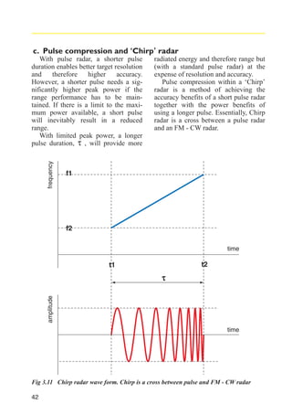
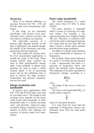
FM-CW radar bandwidth
The bandwidth of an FM - CW radar is
the difference between the start and
finish frequency of the linear frequency
modulation sweep.
Unlike pulse radar, the amplitude of the
FM - CW signal is constant across the
range of frequencies.
Seite 70
A wider bandwidth produces narrower
difference frequency ranges for each
echo on the frequency spectrum. This
leads to better range resolution in the
same way as with shorter duration pulses with pulse radar.
This is explained in the following diagrams and equations.
frequency
fd =
∆F x 2R
Ts x c
fd
∆F
Ts
R
fd
c
∆F
[Eq. 4.1]
bandwidth
sweep time
distance
difference frequency
speed of light
time
Ts
Fast Fourier Transform
The FAST FOURIER
TRANSFORM produces a
frequency spectrum of all echoes
such as that at fd.
There is an ambiguity ∆fd for each
echo fd.
amplitude
fd
∆fd =
2
Ts
[Eq. 4.2]
∆fd
70
frequency

76. radar_applied_to_level_rb.qxd
15.01.2007
18:46
Seite 71
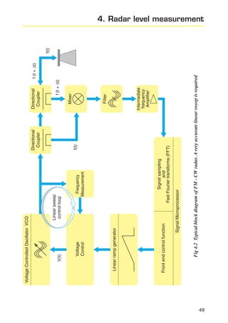
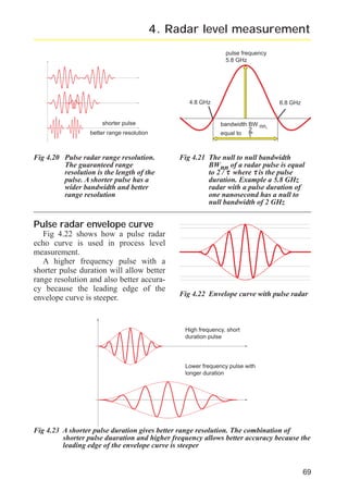
4. Radar level measurement
The ambiguity of the distance R,
is ∆ R
∆fd
fd
∆R
R
=
2
Ts
∆F x 2 R
Ts x c
∆R
R
=
c
∆F x R
∆R
R
∆R
=
=
c
∆F
∆R
R
amplitude
distance
Fig 4.24 to 4.26 - FM - CW range resolution
[Eq. 4.3]
From equation 4.3, it can be seen
that with an FM - CW radar the range
resolution ∆R is equal to:-
c
∆F
Therefore, the wider the bandwidth, the
better the range resolution.
Examples:
A linear sweep of 2 GHz has a range
resolution of 150 mm whereas a 1 GHz
bandwidth has a range resolution of
300 mm.
In process radar applications, each
echo on the frequency spectrum is
processed with an envelope curve. The
above equations (Equations 4.1 to 4.3)
show that the Fast Fourier Transforms
(FFTs) in process radar applications do
not produce a single discrete difference
frequency for each echo in the vessel.
Instead they produce a difference frequency range ∆fd for each echo within
an envelope curve. This translates into
range ambiguity.
71

77. radar_applied_to_level_rb.qxd
15.01.2007
18:46
Seite 72
FM - CW frequency spectrum - bandwidth and range resolution
Frequency spectrum - narrow bandwidth of linear sweep
amplitude
envelope curves
around echoes
frequency
Frequency spectrum - wide bandwidth of linear sweep
amplitude
envelope curves
around echoes
frequency
Fig 4.28 Illustration of envelope curve around the frequency spectram of FM - CW
radars. The same four echoes are shown for radar transmitters with different
bandwidths. An improvement in the range resolution is achieved with a wider
bandwidth of the linear sweep
Other influences on accuracy
As we have demonstrated, FM - CW
and PULSE process radar transmitters
use an envelope curve for measurement. A wider bandwidth produces better range resolution. The correspondingly short echo will have a steep slope
and therefore a more accurate measurement can be made. Other influences on
accuracy include signal to noise ratio
and interference.
72
A high signal to noise ratio allows
more accurate measurement while
interference effects can cause a disturbance of the real echo curve leading to
inaccuracies in the measurement.
Choice of antenna and mechanical
installation are important factors in
ensuring that the optimum accuracy is
achieved.

78. radar_applied_to_level_rb.qxd
15.01.2007
18:46
Seite 73
4. Radar level measurement
High accuracy radar
FM - CW radar
High accuracy of the order of
+ 1 mm is generally meaningless in an
active process vessel or a solids silo.
For example, a typical chemical reactor
will have agitators, baffles and other
internal structures plus constantly
changing product characteristics.
Although custody transfer level
measurement applications are not in the
scope of this book, this section discusses how a higher accuracy can be
achieved.
The fundamental requirement for an
accurate FM - CW radar is an accurate
linear sweep of the frequency modulation.
As with the pulse radar, it is possible
to look inside the envelope curve of the
frequency spectrum if the application
has a simple single echo that is characteristic of a liquids storage tank. This is
achieved by measuring the phase angle
of the difference frequency. However,
this is only practical with custody
transfer applications where fast and
expensive processors are used with
temperature and pressure compensation.
Pulse radar
For most process applications, measurement relative to the pulse envelope
curve is sufficient. However, if the liquid level surface is flat calm and the
echo has a reasonable amplitude, it is
possible to look inside the envelope
curve wave packet at the phase of an
individual wave.
However, the envelope curve of a
high frequency radar with a short pulse
duration is sufficiently steep to produce
a very accurate and cost effective level
transmitter for storage vessel applications.
frequency error
f2
f2
t1
Fig 4.30 It is essential that the linear
sweep of the FM - CW radar is
accurately controlled
Fig 4.29 Higher accuracy of pulse radar
level transmitters can be
achieved by looking at the phase
of an individual wave within the
envelope curve. This is only
practical in slow moving storage
tanks
73

79. radar_applied_to_level_rb.qxd
15.01.2007
18:46
Seite 74
Power
Two wire, loop powered radar
Microwave power
Radar is a subtle form of level measurement. The peak microwave power
of most process radar level transmitters
is less than 1 milliWatt. This level of
power is sufficient for tanks and silos
of 40 metres or more.
The average power depends on the
sweep time and sweep repetition rate of
FM - CW radar and on the pulse duration and pulse repetition frequency of
pulse radar transmitters.
An increase in the microwave power
will produce higher amplitude echoes.
However, it will produce higher amplitude false echoes and ringing noise
as well as a higher amplitude echoes
off the product surface. The average
microwave power of a Pulse radar can
be as little as 1 microWatt.
Pulse radar
The low energy requirements of
pulse radar enabled the first ever two
wire, loop powered, intrinsically safe
radar level transmitter to be introduced
to the process industry in mid-1997.
The VEGAPULS 50 series of pulse
radar transmitters have proved to be
very capable in difficult process conditions. The performance of the two wire,
4 to 20 mA, sensors is equal to the four
wire units that preceded them.
The pulse microwave module only
needs a 3.3 volt power supply with
a maximum power consumption of
50 milliWatts. This drops down to
5 milliWatts when it is in stand-by
mode. The difference between the two
wire pulse and the four wire pulse is
that the two wire radar sends out bursts
of pulses and updates the output about
once every second. The four wire sends
out pulses continuously and updates
seven times a second.
With high quality electronics, the
complete 24 VDC, 4 to 20 mA transmitter is capable of operating at only
14 VDC. This allows it to directly
replace existing two wire sensors.
Processing power
FM - CW radars need a high level of
processing power in order to function.
This processing power is used to calculate the FFT algorithms that produce
the frequency spectrum of echoes.
The requirement for processing power
has restricted the ability of FM - CW
radar manufacturers to make a reliable
two wire, intrinsically safe radar transmitter.
Pulse radar transmitters work in the
time domain without FFT analysis and
therefore they do not need powerful
processors for this function.
Safety
The low power output from
microwave radar transmitters means
that they are an extremely safe method
of level measurement.
74
Pulsed FM - CW
The low power requirements of
pulse radar have allowed two wire
radar to become sucessful. FM - CW
radar requires processing power and
time for the FFT's to be calculated.
Power saving has been used to produce
a ‘pulsed’ FM - CW radar. However,
this device is limited to simple storage
applications because the update time is
too long and the processing too limited
for arduous process applications.

80. radar_applied_to_level_rb.qxd
15.01.2007
18:46
Seite 75
4. Radar level measurement
Summary of radar level techniques
FM - CW (frequency modulated continuous wave) radar
· Indirect method of level measurement
· Requires Fast Fourier Transform (FFT) analysis to convert signals into a frequency spectrum
· FFT analysis requires processing power and therefore practical FM - CW
process radars have to be four wire and not two wire loop powered
· FM - CW radars are challenged by large numbers of multiple echoes (caused
by the parabolic effects of horizontal cylindrical or dished topped vessels)
PULSE radar
· Direct, time of flight level measurement
· Uses a special sampling technique to produce a time expanded intermediate
frequency signal
· The intermediate frequency is produced in hardware and does not require FFT
analysis
· Low processing power requirement mean that practical and very capable two
wire, loop powered, intrinsically safe pulse radar can be used in some of the
most challenging process level applications
75

81. Contents
Foreword
Acknowledgement
Introduction
ix
xi
xiii
Part I
1. History of radar
2. Physics of radar
3. Types of radar
1. CW-radar
2. FM - CW
3. Pulse radar
1
13
33
33
36
39
Part II
4. Radar level measurement
1. FM - CW
2. PULSE radar
3. Choice of frequency
4. Accuracy
5. Power
47
48
54
62
68
74
5. Radar antennas
1. Horn antennas
2. Dielectric rod antennas
3. Measuring tube antennas
4. Parabolic dish antennas
5. Planar array antennas
Antenna energy patterns
77
81
92
101
106
108
110
6. Installation
A. Mechanical installation
1. Horn antenna (liquids)
2. Rod antenna (liquids)
3. General consideration (liquids)
4. Stand pipes & measuring tubes
5. Platic tank tops and windows
6. Horn antenna (solids)
B. Radar level installation cont.
1. safe area applications
2. Hazardous area applications
115
115
115
117
120
127
134
139
141
141
144

82. 5. Radar antennas
The function of an antenna in a radar
level transmitter is to direct the maximum amount of microwave energy
towards the level being measured and
to capture the maximum amount of
energy from the return echoes for
analysis within the electronics.
Antennas for level measurement
come in five basic forms:
· Horn (cone) antenna
· Dielectric rod antenna
· Measuring tube antenna
(stand pipes/ bypass tubes etc.)
· Parabolic reflector antenna
· Planar array antenna
Horn antennas and dielectric rod
antennas are already commonly used
within process level measurement. We
will be discussing how these designs
have been developed for increasingly
arduous process conditions and how
antenna efficiencies have been
improved. The horn antenna and versions of the dielectric rod antenna are
also used in measuring tube applications within the process industry.
Parabolic antennas and planar array
antennas have been applied to fiscal
measurement radar systems rather than
for level measurement within process
vessels. We will discuss the design of
these antennas although at present their
use in process vessels is limited.
Antenna basics
An important aspect of an antenna is
directivity. Directivity is the ability of
the antenna to direct the maximum
amount of radiated microwave energy
towards the liquid or solid we wish to
measure.
No matter how well the antenna is
designed, there will be some
microwave energy being radiated in
every direction. The goal is to maximise the directivity.
Fig 5.1 shows the pattern of radiated
energy from a typical horn antenna.
This is a 250 mm (10") horn antenna
operating at a frequency of 5.8 GHz.
The measurements are made some
distance from the antenna in what is
called the far field zone. It is clear that
most of the energy is contained within
the main lobe, but also there is a reasonable amount of energy contained
within the various side lobes.
Technical information and sales literature on radar level transmitters
quote beam angles for different antennas. Clearly there is not a tight beam.
The convention is to measure the angle
at which the microwave energy has
reduced to 50 percent of the value at
the central axis of the beam.
This is quoted in decibels:the - 3dB point.
77

83. Farfield E_Abs (Theta); Phi=90,0 deg.
90
Max.: 20,4 dB
120
60
30
150
180
0
10
20
150
30
0
30
120
main lobe direction
: 0,0 deg.
angular width (3dB) : 14,9 deg.
side lobe suppression : 21,6 dB
60
90
Extent of measured microwave energy showing
main lobe and side lobes
The - 3 dB point is the beam angle i.e. the energy
has reduced to 50%
Side lobe energy
Fig 5.1 Typical radiation pattern from a radar level transmitter
Radiation patterns of different antennas and radar frequencies are compared at the
end of this chapter.
78

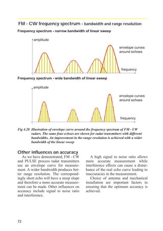
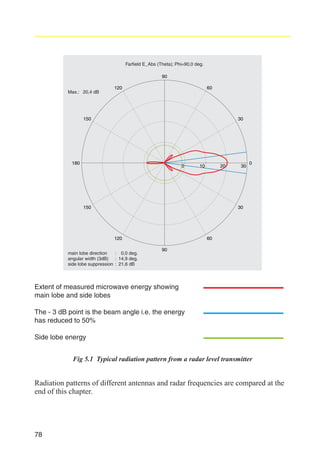
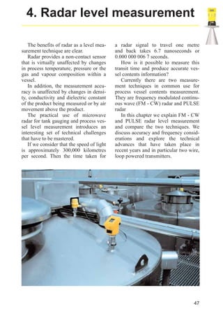
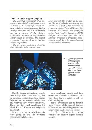
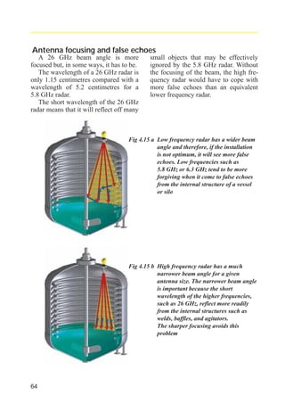
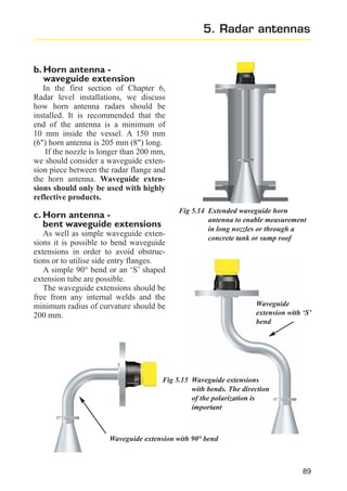
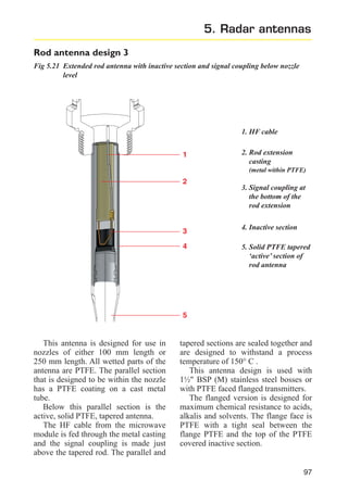
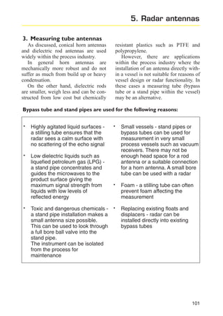
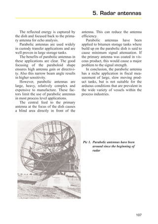
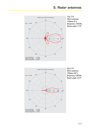
84. 5. Radar antennas
A measure of how well the antenna
is directing the microwave energy is
called the ‘antenna gain’.
Antenna gain is a ratio between the
power per unit of solid angle radiated
by the antenna in a specific direction to
the power per unit of solid angle if the
total power was radiated isotropically,
that is to say, equally in all directions.
isotropic power
directional power
Isotropic equivalent with total power
radiating equally in all directions
Directional power from antenna
Fig 5.2 Illustration of antenna gain
Antenna gain ‘G’ can be calculated as follows:
G = ηx
(
πxD
λ
2
)
= ηx
4π x A
λ2
[Eq. 5.1]
Where
The aperture efficiencies of radar
level antennas are typically between
η = 0.6 and η = 0.8.
D = antenna diameter.*
It is clear from equation 5.1 that
the directivity improves in proportion
A = antenna area.*
to the antenna area. At a given freλ = microwave wavelength * quency, a larger antenna has a narrower beam angle
η = aperture efficiency
* must be same units
79

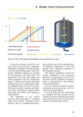
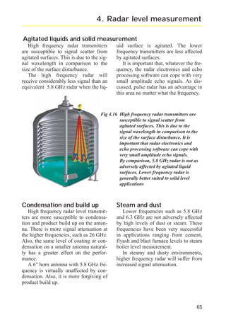
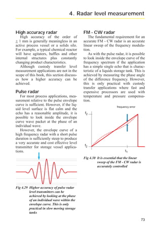
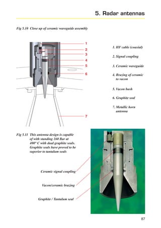
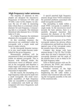
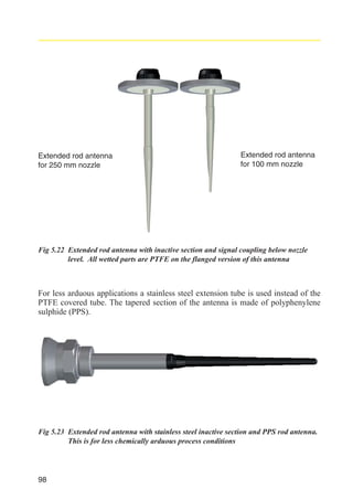
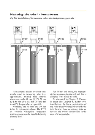
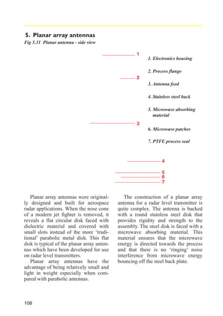
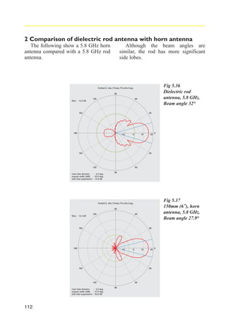
85. Also, we can see that the antenna
gain and hence directivity is inversely
proportional to the square of the wavelength.
For a given size of antenna the beam
angle will become narrower at higher
frequencies (shorter wavelengths). For
example the beam angle of a 5.8 GHz
radar with a 200 mm (8") horn antenna
is almost equivalent to a 26 GHz radar
with a 50 mm (2") horn antenna. This
Beam angle
φ
=
means that a 26 GHz antenna is lighter
and easier to install for the same beam
angle. However, as discussed in
Chapter 4, this is not the whole story
when choosing the right transmitter for
an application.
For a standard horn antenna the
beam angle φ, that is the angle to the
minus 3 dB position, can be calculated
using equation 5.2.
70° x
λ
D
[Eq. 5.2]
The following graph shows horn antenna diameter versus beam angle for the
most common radar frequencies,
5.8 GHz, 10 GHz and 26 GHz.
Antenna beam angles (diameter / frequency)
beam angle in degrees (-3dB)
80
5.8 GHz
10 GHz
60
26 GHz
40
20
0
50
75
100
125
150
175
200
225
250
antenna diameter, mm
Fig 5.3 Graph showing relation between horn antenna diameter and beam angle for
5.8 GHz, 10Ghz and 26GHz radar
80

86. 5. Radar antennas
1. Horn antennas
The metallic horn antenna or cone
antenna is well proven for process level
applications. The horn is mechanically
robust and in general it is virtually
unaffected by condensation and product build up, especially at the lower
radar frequencies such as 5.8 GHz.
There are variations in the internal
design of horn antennas. The
microwaves that are generated within
the microwave module are transmitted
down a high frequency cable for encoupling into a waveguide. The metal
waveguide then directs the microwaves
towards the horn of the antenna. A low
dielectric material such as PTFE,
ceramic or glass is often used within
the waveguide.
At the transition from the waveguide to the horn of the antenna the low
dielectric material is machined to a
pointed cone. The angle of this cone
depends on the dielectric constant of
the material. For example, ceramic has
a sharper angle than PTFE.
The microwaves are emitted from
this pointed cone in a controlled way
and are then focused towards the target
by the metal horn.
After reflection from the product
surface, the returning echoes are
collected within the horn antenna for
processing within the electronics.
Fig 5.4 The transition of
microwaves from the low
dielectric waveguide into the
metallic horn where they are
focused towards the product
being measured
81

87. Horn antenna design 1
Fig 5.5
1. HF Cable
1
2
3
4
5
6
7
8
2. Signal coupling
3. Waveguide (air filled)
Transition rectangular to circular
cross section
4. PTFE transition
5. Glass waveguide
9
6. Metallic grid
7. Seal between glass
and PTFE
8. PTFE cone
9. Metal horn antenna
In this first design of horn antenna
the HF cable signal coupling is into an
air filled waveguide with a rectangular
cross section. The microwaves are
directed towards the antenna. There is a
transition from rectangular to circular
cross section. At this point the waveguide changes to PTFE with a ¼ wavelength step design. The waveguide is
then glass filled until it reaches the
inside of the antenna horn where it
changes to a PTFE cone for the impedance matching into the vapour space in
the horn
This PFTE cone in combination with
the metallic horn focuses the
microwaves towards the target.
82
An antenna of this design is capable
of withstanding process temperatures
up to 250° C and up to 300 Bar.
A potential problem with the design
is the sealing between the PTFE and
glass on the process side. The thermal
expansion of glass and PTFE are different and it is possible for condensation
to get between the glass and PTFE and
to affect the transmission and receipt of
the microwave signals.
The explosion proof design requires
metallic grid around the glass of the
waveguide at the joint between the
housing casting and the flange casting.

88. 5. Radar antennas
Horn antenna design 2
Fig 5.6
1. HF cable
2. Signal coupling
1
3. Waveguide
(PTFE filled)
2
3
4
5
4. Process seals Viton
or Kalrez
5. PTFE cone
6. Metallic horn
antenna
6
With this antenna design, the HF
cable is encoupled into the PTFE material inside the waveguide. The metal
waveguide is welded to the flange and
there are two process seals between the
metal waveguide and the PTFE. These
seals protect the signal coupler from
the process. This seal material can be
Viton for stainless steel horn antennas
or Kalrez for Hastelloy C horn antennas.
There is a continuous transition for
the microwaves within a single piece of
PTFE which is machined into a cone
form for the transition into the horn
antenna. The PTFE cone and the metallic conical horn focus the microwaves
and collect the return signals in the
usual manner.
An antenna of this design is capable
of withstanding a process temperature
of 200° C + and a process pressure of
40 Bar.
This antenna design can also be used
on very high temperature, ambient
pressure applications with air or nitrogen gas cooling of the antenna.
83

89. Horn antenna design 2a
Fig 5.7 Very high temperature, ambient pressure applications.
Air/nitrogen cooling through flange
1. HF cable
1
2. Signal coupling
2
3. Waveguide
(PTFE filled)
3
4
4. Tappings for
air/nitrogen keeps
antenna area cool
Air / N2
5. Metallic horn
antenna
5
This adaptation of the previous
antenna allows the antenna to be cooled
with air or nitrogen gas.
This is achieved by drilling two
holes, 180° apart, laterally from the
flange edge into the horn antenna next
to the PTFE cone. The flow of air or
nitrogen prevents hot gases from
affecting the PTFE and the viton seal
and it effectively cools the entire flange
and horn area.
This technique has been used successfully with very high temperatures,
including 1500° C + in the steel industry with applications such as blast
84
furnace burden level and molten iron
ladle levels. The microwaves are unaffected by the air movement within the
horn area.
In addition to cooling, this air purging technique is also used for solids
applications where very high levels of
conductive dust, such as carbon, heavily coat the inside of the horn and cause
signal attenuation.
Water purging has also been used
where heavy product build up is
expected.

90. 5. Radar antennas
Horn antenna design 3
Fig 5.8 Special enamel coated antenna
1
2
1. Signal coupling
2. PTFE waveguide
3
4
5
3. PTFE flange face
4. PTFE seal
6
5. Lapped flange
7
6. Steel internals of
horn antenna
7. Enamelled coating
This antenna is also a development
of the antenna design in Fig 5.6.
The waveguide, PTFE transition
cone and process flange are standard.
The face of the flange is all PTFE.
The difference is in the application
of a special enamel (glass) coated horn
that provides excellent process materials compatibility without resorting to
more expensive metals such as
Tantalum.
The external dimensions of the
antenna represent a simple cylinder.
The internal dimensions of the antenna
are identical to a standard horn antenna
(150 mm (6")) is illustrated. At the bottom of the antenna there is a gradual lip
between the external cylinder and the
internal horn.
The top of the cylinder has a flange
for sealing between the PTFE transition
cone and the process flange and also
between the glassed antenna and the
vessel nozzle. External studs hold the
enamel antenna to the process flange
and PTFE seals are used to provide
internal sealing.
The antenna is manufactured from
carbon steel with blue enamel coating
which is identical to the enamel found
in glass lined vessels. It provides the
efficiency benefits of a horn antenna
with first class materials compatibility.
85

91. Horn antenna design 4
Fig 5.9 High temperature / high pressure antenna with ceramic waveguide
1
2
3
4
1. Connection to HF
cable from
microwave module
2. Coaxial tube to
signal coupling
3. Signal coupling in
ceramic waveguide
4.Vacon/ceramic
brazing seal
5
5. Graphite seal
6
6. Ceramic waveguide
cone
The above antenna has been
designed with both high temperature
and high pressure in mind. The
mechanical strength and sealing ability
of PTFE degrades at elevated temperature and is therefore limited to about
200° C.
This special design of radar has
a chemically and thermally stable
ceramic (Al2O3) waveguide within a
stainless steel or Hastelloy C horn
antenna and flange. The ceramic
waveguide is fused to a ‘vacon’ steel
bush using a special brazing technique.
‘Vacon’ is used because it has a
coefficient of thermal expansion that is
similar to ceramic, whereas normal
86
stainless steel expands more than twice
as much as ceramic. A double graphite
seal is fitted on the process side of the
‘vacon’ bush. The entire waveguide
assembly is laser welded to ensure that
the transmitter is gas tight and that
differential thermal expansion is
negligible.
In order to withstand constant process temperatures of 400° C, the electronics housing of the radar is mechanically isolated from the high process
temperature by a temperature extension
tube. The microwave module is connected via the HF cable and an air
coaxial tube to the signal coupler in the
ceramic waveguide.

92. 5. Radar antennas
Fig 5.10 Close up of ceramic waveguide assembly
1
2
3
1. HF cable (coaxial)
2. Signal coupling
4
5
3. Ceramic waveguide
6
4. Brazing of ceramic
to vacon
5. Vacon bush
6. Graphite seal
7. Metallic horn
antenna
7
Fig 5.11 This antenna design is capable
of with standing 160 Bar at
400° C with dual graphite seals.
Graphite seals have proved to be
superior to tantalum seals
Ceramic signal coupling
Vacon/ceramic brazing
Graphite / Tantalum seal
87

93. Adapting horn antenna radars
a. Measurement through a PTFE window
Another possible variation of a horn
antenna radar is measurement through
a low dielectric window. We have discussed Hastelloy, Tantalum and the
special enamel coated horn antenna.
However, if a liquid is being measured
and it is conductive or has a dielectric
constant of more that εr = 10, then it is
possible to measure through a low
dielectric window or lens.
Some antennas are manufactured
with a PTFE window as part of the
construction.
Antenna housing
Horn antenna
Process flange
PTFE window
Fig 5.12 Horn antenna radar is constructed with a metal housing around the antenna
and a PTFE process ‘window’
Fig 5.13 Variations of this design include the use of cone shaped windows. The cone can
point towards the horn or towards the process
88

94. 5. Radar antennas
b. Horn antenna waveguide extension
In the first section of Chapter 6,
Radar level installations, we discuss
how horn antenna radars should be
installed. It is recommended that the
end of the antenna is a minimum of
10 mm inside the vessel. A 150 mm
(6") horn antenna is 205 mm (8") long.
If the nozzle is longer than 200 mm,
we should consider a waveguide extension piece between the radar flange and
the horn antenna. Waveguide extensions should only be used with highly
reflective products.
c. Horn antenna bent waveguide extensions
As well as simple waveguide extensions it is possible to bend waveguide
extensions in order to avoid obstructions or to utilise side entry flanges.
A simple 90° bend or an ‘S’ shaped
extension tube are possible.
The waveguide extensions should be
free from any internal welds and the
minimum radius of curvature should be
200 mm.
Fig 5.14 Extended waveguide horn
antenna to enable measurement
in long nozzles or through a
concrete tank or sump roof
Waveguide
extension with ‘S’
bend
Fig 5.15 Waveguide extensions
with bends. The direction
of the polarization is
important
Waveguide extension with 90° bend
89

95. High frequency radar antennas
The majority of antennas in this
chapter are designed for microwave
frequencies of between 5.8 GHz and
10 GHz. Later in this chapter, we discuss the use of radar in measuring
tubes where there is a minimum critical
diameter for each frequency. A measuring tube is a waveguide. The minimum
theoretical tube diameter for a 5.8 GHz
radar is 31 mm.
At a higher frequency the minimum
diameter of a waveguide is smaller.
At this minimum diameter, the
microwaves are established within the
waveguide with a single mode and
hence a single velocity.
As the waveguide diameter increases in size, more modes become established for the given frequency.
Measurement problems will be
encountered if there are multiple modes
within an antenna waveguide. This is
because with different modes the
microwaves travel at different velocities in the waveguide and therefore a
single target will reflect more than one
return echo. Measurement will become
inaccurate or impossible.
For this reason, the encoupling of a
high frequency radar must be made into
a small waveguide. The small waveguide assemblies of high frequency
radar are susceptible to contamination
by condensation and build up when
compared with lower frequencies such
as 5.8 GHz.
90
A special patented high frequency
antenna design from VEGA minimises
the potential problems associated with
small waveguide assemblies.
The encoupling is made within a
small PTFE waveguide to establish a
single mode. As the microwaves travel
towards the horn antenna, there is a
carefully designed transition that
increases the diameter of the PTFE
waveguide while maintaining the single
mode.
The increased diameter of the PTFE
waveguide reduces the adverse effects
of condensation and build up where the
tapered cone of the waveguide enters
the metallic horn of the antenna.
Compare this design with horn
antenna design 2, Fig 5.6. The 5.8 GHz
radar does not need a transition in the
waveguide diameter and the angle of
the metallic horn is not as sharp as for
the high frequency radar.
Viton or Kalrez process seals are fitted between the PTFE and stainless
steel body of the waveguide.
Extended versions of the high
frequency antenna design involve
lengthening the HF cable within a
stainless steel extension tube and welding the waveguide assembly to the end
of the extension tube.

96. 5. Radar antennas
Fig 5.16 High frequency (26GHz) horn antenna design
1. HF cable from
microwave module
2. Signal coupling into
smaller diameter PTFE
waveguide assembly
1
2
3
4
5
6
3. Carefully designed
transition from small
diameter to larger
diameter without
affecting the waveguide
mode
4. Viton or Kalrez process
seals between PTFE and
stainless steel of the
waveguide
5. Cone shape of PTFE
waveguide for the
transition into the
metallic horn of the
antenna
6. Metallic horn antenna
of high frequency radar.
It has a sharper angle
than the lower frequency
radars
91

97. 2. Dielectric rod antennas
The dielectric rod antenna is an
extremely useful option when applying
radar level technology to modern
process vessels. Dielectric rods can be
used in vessel nozzles as small as
40 mm (1½") and they are manufactured from PP, PTFE or ceramic wetted
parts.
This means that, normally, radar
level transmitters can be retro-fitted
into existing tank nozzles and they
have low cost materials compatibility
with most aggressive liquids including
acids, alkalis and solvents.
The design of dielectric rod antennas
has been refined in recent years.
Essentially the microwaves are fed
from the microwave module through an
HF cable to a signal coupler in the
waveguide. As with the horn antenna
the waveguide can be air filled or filled
with a low dielectric material such as
PTFE .
The
waveguide
feeds
the
microwaves to the antenna. The
microwaves pass down the parallel
section of the rod until they reach the
tapered section of the rod. The tapered
section of the rod acts like a lens and it
focuses the microwaves towards the
product being measured. The size and
shape of the dielectric rod depends on
the frequency of the microwaves being
transmitted.
92
The reflected echoes are captured in
a similar fashion for processing by the
radar electronics.
Rod antennas should only be used
on liquids and slurries and not on powders and granular products.
There are some important considerations when applying rod antenna
radars.
First of all, the tapered section of the
rod must be entirely within the vessel.
If the tapered section is in a nozzle,
it will cause ‘ringing’ noise that will
effectively blind the radar. This is
explained more fully in Chapter 6.
Also, it can be seen from Fig 5.17
that the microwaves rely on the rod
antenna being clean. If a rod antenna is
coated in viscous, conductive and adhesive products, the antenna efficiency
will deteriorate very quickly.
With the horn antenna product build
up is not a particular problem.
However, product build up works
against the reliable functioning of a rod
antenna radar.

98. 5. Radar antennas
Fig 5.17 Dielectric rod antenna
The microwaves travel down the inactive
parallel section of the rod towards the
tapered section .
The tapered section of the rod focuses the
microwaves toward the liquid being
measured .
It is very important that all of the tapered
section of the rod must be inside the vessel
It is not good practice to allow a rod
antenna to be immersed in the product
If a rod antenna is coated in viscous,
conductive and adhesive product, the
antenna efficiency will deteriorate
93

99. Rod antenna design 1
Fig 5.18 Rod antenna for short process nozzles
1
2
3
1. HF cable
2. Process connection
PVDF boss
4
3. Signal coupling
within PTFE/PP
filled waveguide
4. Inactive section
with metallic waveguide, PTFE/PP
inner and outer
parts
5. Solid PTFE/PP
active tapered
section of antenna
focuses the
microwaves towards
the product surface
5
This rod antenna is a simple and low
cost design that provides a radar level
transmitter with good materials compatibility. It is ideal for vented and low
pressure vessels such as acid and alkali
tanks. It is designed for use in short
1½" BSP / NPT process nozzles. The
nozzle height should not exceed 60 mm
(2½").
The process connection is a 1½"
PVDF boss and the antenna is
polypropylene (PP) or PTFE.
94
The HF cable from the microwave
module is coupled into PTFE/PP inside
a metallic tube that acts as a waveguide. This metallic tube is totally
enclosed within the PTFE/PP parallel
section of the antenna. The microwaves
pass down the metallic waveguide
directly to the tapered section of the
antenna where they are focused
towards the product being measured.

100. 5. Radar antennas
Rod antenna design 2
Fig 5.19 Rod antenna with solid PTFE extendible rod
1. HF cable
1
2
3
4
5
2. Signal coupling
3. Air waveguide
4. PTFE cone
5. Process connection
6
7
With this design of rod antenna the
signal coupling is into an air filled
waveguide. The microwaves are directed towards the antenna. There is a transition to PTFE via a cone shaped element. The microwaves continue
through the PTFE waveguide to the
solid PTFE dielectric rod. The tapered
section of the rod focuses the
microwaves towards the product being
measured.
6. Solid PTFE parallel
section length can
be extended
7. Solid PTFE tapered
section
If this type of antenna is to be used
in a long nozzle, the parallel section of
the solid rod is extended to ensure that
the tapered section is entirely within
the vessel.
An extended, solid PTFE rod antenna can suffer from ‘ringing’ noise
caused by microwave leakage from the
parallel section resonating within the
nozzle. See Fig 5.20.
95

101. Fig 5.20 Extended rod antenna in solid PTFE. This design can suffer from ‘ringing’
noise caused by leakage of microwave energy from the parallel section of the
solid PTFE rod resonating in the vessel nozzle
In theory, the microwaves should
travel within the parallel section for the
entire length until it reaches the tapered
section. However, in practice, some of
the microwave energy escapes from the
parallel sides.
Some solid PTFE rod antennas
are supplied with screw - on extendible
antennas.
In addition to the ‘ringing’ noise
problem described, this design can suffer from condensation forming between
the rod sections causing signal
attenuation.
96
Also the PTFE expands at elevated
temperatures and under certain process
conditions it is possible for the rod sections to detach.
The potential problems of solid
PTFE rod antennas have been solved
by the latest designs. It is important to
have a completely inactive parallel section within a vessel nozzle. This is
achieved by special screening or signal
coupling beyond the nozzle.

102. 5. Radar antennas
Rod antenna design 3
Fig 5.21 Extended rod antenna with inactive section and signal coupling below nozzle
level
1. HF cable
1
2. Rod extension
casting
(metal within PTFE)
2
3. Signal coupling at
the bottom of the
rod extension
3
4. Inactive section
4
5. Solid PTFE tapered
‘active’ section of
rod antenna
5
This antenna is designed for use in
nozzles of either 100 mm length or
250 mm length. All wetted parts of the
antenna are PTFE. The parallel section
that is designed to be within the nozzle
has a PTFE coating on a cast metal
tube.
Below this parallel section is the
active, solid PTFE, tapered antenna.
The HF cable from the microwave
module is fed through the metal casting
and the signal coupling is made just
above the tapered rod. The parallel and
tapered sections are sealed together and
are designed to withstand a process
temperature of 150° C .
This antenna design is used with
1½" BSP (M) stainless steel bosses or
with PTFE faced flanged transmitters.
The flanged version is designed for
maximum chemical resistance to acids,
alkalis and solvents. The flange face is
PTFE with a tight seal between the
flange PTFE and the top of the PTFE
covered inactive section.
97

103. Extended rod antenna
for 250 mm nozzle
Extended rod antenna
for 100 mm nozzle
Fig 5.22 Extended rod antenna with inactive section and signal coupling below nozzle
level. All wetted parts are PTFE on the flanged version of this antenna
For less arduous applications a stainless steel extension tube is used instead of the
PTFE covered tube. The tapered section of the antenna is made of polyphenylene
sulphide (PPS).
Fig 5.23 Extended rod antenna with stainless steel inactive section and PPS rod antenna.
This is for less chemically arduous process conditions
98

104. 5. Radar antennas
Rod antenna design 4
Fig 5.24 Extended rod antenna with metallic grid waveguide extension within carbon
impregnated PTFE inactive rod. Tapered active section of virgin PTFE
1. HF cable
1
2. Signal coupling
2
3
4
5
3. PTFE waveguide
6
7
4. Screwed connection
5. Carbon impregnated
PTFE antenna parallel
section and flange face
6. Internal metal grid acts
as extended waveguide
and prevents microwave
leakage from the
parallel section of the
antenna
7. PTFE waveguide
8
This design of dielectric rod antenna
is for use with flanged process connections.
The HF cable is connected into a
PTFE filled waveguide which directs
the microwave energy towards the rod
antenna. There is a PTFE male screwed
fitting at the end of the waveguide
within the process flange. The fabricated, one piece, rod antenna screws on to
this connection.
The antenna flange facing and the
parallel section of the antenna have carbon impregnated PTFE wetted parts.
Inside the parallel section of the rod
there is a tubular metallic grid that acts
8. Virgin PTFE tapered
antenna
as an extension to the waveguide.
Inside the grid the waveguide is virgin
PTFE, outside the grid the PTFE is carbon impregnated.
At the end of the parallel section,
there is a transition into a solid PTFE
tapered rod which provides the impedance matching and focusing of the
microwaves towards the product being
measured.
This antenna has the option for
100 mm or 250 mm nozzle lengths. As
already discussed, the tapered section
must be entirely within the vessel.
99

105. Rod antenna design 5
Fig 5.25 This is a high temperature ceramic rod antenna design. There is temperature
separation between the electronics and the signal coupling (similar to the high
temperature horn antenna Fig 5.10). The ceramic rod has a sharper taper than
the equivalent PTFE rod
1
2
3
4
1. Signal coupling
2. Ceramic waveguide
3. Process seal (graphite or
tantalum)
4. Active tapered ceramic
rod
Rod antennas are available with the
dielectric rod manufactured from
ceramic (Al2O3).
Ceramic has good chemical and
thermal resistance. However, care must
100
be taken when installing ceramic rods
because they are brittle and prone to
accidental damage.

106. 5. Radar antennas
3. Measuring tube antennas
As discussed, conical horn antennas
and dielectric rod antennas are used
widely within the process industry.
In general horn antennas are
mechanically more robust and do not
suffer as much from build up or heavy
condensation.
On the other hand, dielectric rods
are smaller, weigh less and can be constructed from low cost but chemically
resistant plastics such as PTFE and
polypropylene.
However, there are applications
within the process industry where the
installation of an antenna directly within a vessel is not suitable for reasons of
vessel design or radar functionality. In
these cases a measuring tube (bypass
tube or a stand pipe within the vessel)
may be an alternative.
Bypass tube and stand pipes are used for the following reasons:
·
·
·
Highly agitated liquid surfaces a stilling tube ensures that the
radar sees a calm surface with
no scattering of the echo signal
Low dielectric liquids such as
liquefied petroleum gas (LPG) a stand pipe concentrates and
guides the microwaves to the
product surface giving the
maximum signal strength from
liquids with low levels of
reflected energy
Toxic and dangerous chemicals a stand pipe installation makes a
small antenna size possible.
This can be used to look through
a full bore ball valve into the
stand pipe.
The instrument can be isolated
from the process for
maintenance
·
·
·
Small vessels - stand pipes or
bypass tubes can be used for
measurement in very small
process vessels such as vacuum
receivers. There may not be
enough head space for a rod
antenna or a suitable connection
for a horn antenna. A small bore
tube can be used with a radar
Foam - a stilling tube can often
prevent foam affecting the
measurement
Replacing existing floats and
displacers - radar can be
installed directly into existing
bypass tubes
101

107. Measuring tube radar 1 - horn antennas
Fig 5.26 Installation of horn antenna radars into stand pipes or bypass tube
DN50
DN80
DN100
∅ 50
∅ 80
∅ 100
Horn antenna radars are most commonly used in measuring tube level
applications. Stilling tube internal
diameters can be 40 mm (1 ½"), 50 mm
(2"), 80 mm (3"), 100 mm (4") and 150
mm (6"). Larger tubes are possible.
Normally, the 40 mm and 50 mm
tubes do not require a horn. The PTFE
or ceramic waveguide impedance
matching cone can be installed directly
into the tube.
102
DN150
∅ 150
For 80 mm and above, the appropriate horn antenna is attached and this is
designed to fit inside the tube.
As discussed in Chapter 2, Physics
of radar and Chapter 6, Radar level
installations, the linear polarization of
the radar must be directed towards the
tube breather hole or mixing slots, or
towards the process connections in the
case of a bypass tube.

108. 5. Radar antennas
Measuring tube radar 2 - offset rod antennas
Fig 5.27 Offset rod antenna for use on 50 mm and 80 mm measuring tubes
1
1. HF cable
2. Signal coupling
3. PTFE faced flange
4. Offset short solid PTFE
rod antenna
2
3
4
The standard length dielectric rod
antennas should not be installed within
measuring tubes. There is a high level
of ‘ringing’ noise which severely
reduces the efficiency of the antenna.
However, a special design of short,
offset rod antenna can be used on small
diameter tubes (50 mm and 80 mm).
This design is similar in construction
to rod antenna design 3. All wetted
parts are in PTFE and the short antenna
is off centre. This asymmetric design
produces improved signal to noise
ratios within a measuring tube.
103

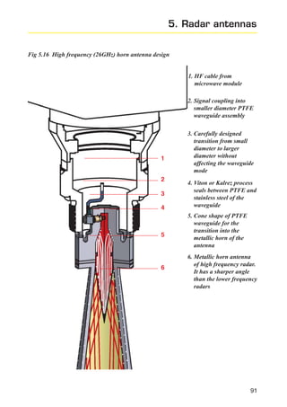
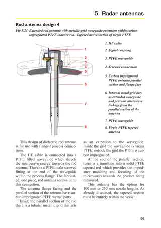
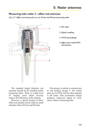
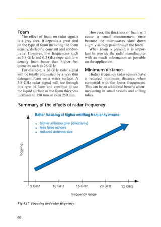
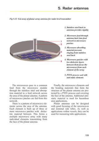
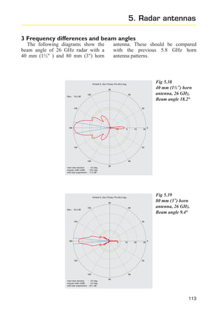
109. Microwave velocity within measuring tube
The speed of microwaves within a
measuring tube is apparently slower
when compared to the velocity in free
space. The degree to which the running
time slows down depends on the diameter of the tube and the wavelength of
the signal.
cwg = co x
{
1-
2
}
λ
( 1.71d )2
[Eq. 5.3]
The microwaves bounce off the
sides of the tube and small currents are
induced in the walls of the tube. For a
circular tube, or waveguide, the
velocity change is calculated by the
following equation :
cwg
co
λ
d
is the speed of microwaves in
the measuring tube / waveguide
is the speed of light in free
space
is the wavelength of the
microwaves
is the diameter of the measuring tube
Fig 5.28 The transit time of microwaves
is slower within a stilling tube.
This effect must be compensated
within the software of the radar
level transmitter
104

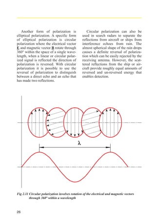
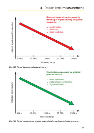
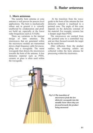
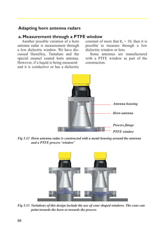
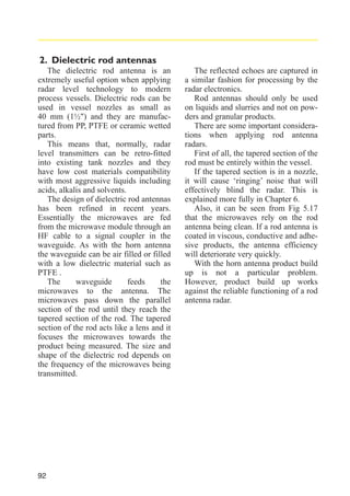
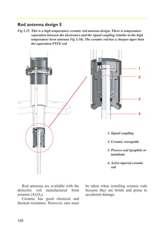
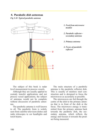
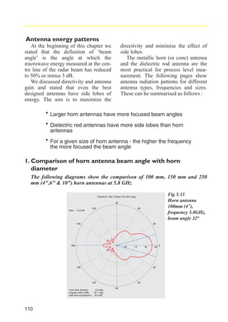
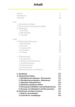
110. 5. Radar antennas
There are different modes of propagation of microwaves within a waveguide. However, an important value is
the minimum diameter of pipe that will
allow microwave propagation.
The value of the critical diameter,
dc , depends upon the wavelength λ of
the microwaves: The higher the frequency of the microwaves, the smaller
the minimum diameter of measuring
tube that can be used.
dc =
Equation 5.4 shows the relationship
between critical diameter and wavelength. For example, 5.8 GHz has a
wavelength λ of ~ 52 mm. The minimum theoretical tube diameter is
dc = 31 mm
With a frequency of 26 GHz, a
wavelength of 11.5 mm, the minimum
tube diameter is dc = 6.75 mm. In practice the diameter should be higher. The
diameter for 5.8 GHz should be at least
40 mm.
λ
1.71
[Eq. 5.4]
% speed of light, c
100
80
60
40
20
0
0.6 0.8 1.0 1.2 1.4 1.6 1.8 2.0 2.2 2.4 2.6 2.8 3.0
Tube diameter / wavelength, d / λ
Fig 5.29 Graph showing the effect of measuring tube diameter on the propagation speed
of microwaves
Higher frequencies such as 26 GHz
will be more focused within larger
diameter stilling tubes. This will minimise false echoes from the stilling tube
wall.
The installation requirements of
radar level transmitters in measuring
tubes are covered in the next chapter.
105

111. 4. Parabolic dish antennas
Fig 5.30 Typical parabolic antenna
1. Feed from microwave
module
2. Parabolic reflector secondary antenna
1
3. Primary antenna
4. Focus of parabolic
reflector
2
3
4
The subject of this book is radar
level measurement in process vessels.
Although they are usually applied to
custody transfer applications and not
process vessel applications, the subject
of antennas would not be complete
without discussion of parabolic antennas.
The parabolic antenna is well known
to all. The parabolic form is widely
seen from satellite television dishes and
radio telescopes to car headlights and
torch beams.
106
The main structure of a parabolic
antenna is the parabolic reflector dish.
This is usually of stainless steel construction and is designed to focus the
microwaves as accurately as possible.
The microwaves are fed through the
centre of the dish to the primary antenna that is in front of the dish at the
focus. The microwave energy is transmitted from the primary antenna back
towards the parabolic dish, the secondary antenna, which reflects the
energy and focuses it towards the product being measured.

112. 5. Radar antennas
The reflected energy is captured by
the dish and focused back to the primary antenna for echo analysis.
Parabolic antennas are used widely
in custody transfer applications and are
well proven in large storage tanks.
The benefits of parabolic antennas in
these applications are clear. The good
focusing of the paraboloid shape
ensures high antenna gain or directivity. Also this narrow beam angle results
in higher sensitivity.
However, parabolic antennas are
large, heavy, relatively complex and
expensive to manufacture. These factors limit the use of parabolic antennas
in most process level applications.
The central feed to the primary
antenna at the focus of the dish causes
a blind area directly in front of the
antenna. This can reduce the antenna
efficiency.
Parabolic antennas have been
applied to bitumen storage tanks where
build up on the parabolic dish is said to
cause minimum signal attenuation. If
the primary antenna was coated in viscous product, this would cause a major
problem to the signal strength.
In conclusion, the parabolic antenna
has a niche application in fiscal measurement of large, slow moving product tanks, but is not suitable for the
arduous conditions that are prevalent in
the wide variety of vessels within the
process industries.
Pic 1. Parabolic antennas have been
around since the beginning of
radar
107

113. 5. Planar array antennas
Fig 5.31 Planar antenna - side view
1
1. Electronics housing
2. Process flange
2
3. Antenna feed
4. Stainless steel back
5. Microwave absorbing
material
3
6. Microwave patches
7. PTFE process seal
4
5
6
7
Planar array antennas were originally designed and built for aerospace
radar applications. When the nose cone
of a modern jet fighter is removed, it
reveals a flat circular disk faced with
dielectric material and covered with
small slots instead of the more ‘traditional’ parabolic metal dish. This flat
disk is typical of the planar array antennas which have been developed for use
on radar level transmitters.
Planar array antennas have the
advantage of being relatively small and
light in weight especially when compared with parabolic antennas.
108
The construction of a planar array
antenna for a radar level transmitter is
quite complex. The antenna is backed
with a round stainless steel disk that
provides rigidity and strength to the
assembly. The steel disk is faced with a
microwave absorbing material. This
material ensures that the microwave
energy is directed towards the process
and that there is no ‘ringing’ noise
interference from microwave energy
bouncing off the steel back plate.

114. 5. Radar antennas
Fig 5.32 Cut away of planar array antenna for radar level transmitter
1. Stainless steel back to
antenna provides rigidity
1
2
3
4
5
2. Microwave feed through
antenna back into feed
network to microwave
patches
3. Microwave absorbing
material prevents
ringing from stainless
steel back
4. Microwave patches with
low dielectric layers
between them focus the
microwaves from each
element of the array
5. PTFE process seal with
anti-static elements
The microwaves pass in a common
feed from the microwave module
through the stainless steel and absorption material to a feed network across
the area of the planar antenna. A pattern
of microwave patches are fed from this
network.
There is a pattern of microwave elements across the area of the antenna.
Each element is built up of three or
more microwave patches with dielectric material between. This forms a
multiple microwave array with many
individual elements transmitting from
the face of the planar antenna.
Finally, the microwave elements and
the bonding materials that form the
structure of the planar antenna are protected by a PTFE process seal covering
the face of the antenna. Additional antistatic material is used for hazardous
area applications.
Planar antennas can be designed
with good focusing of the microwaves
and minimal side lobes. As well as
applications within vessels, they can be
used for measuring tube applications.
109

115. Antenna energy patterns
At the beginning of this chapter we
stated that the definition of ‘beam
angle’ is the angle at which the
microwave energy measured at the centre line of the radar beam has reduced
to 50% or minus 3 dB.
We discussed directivity and antenna
gain and stated that even the best
designed antennas have side lobes of
energy. The aim is to maximize the
directivity and minimise the effect of
side lobes.
The metallic horn (or cone) antenna
and the dielectric rod antenna are the
most practical for process level measurement. The following pages show
antenna radiation patterns for different
antenna types, frequencies and sizes.
These can be summarised as follows :
· Larger horn antennas have more focused beam angles
· Dielectric rod antennas have more side lobes than horn
antennas
· For more focusedofthe beam angle- the higher the frequency
a given size horn antenna
the
1. Comparison of horn antenna beam angle with horn
diameter
The following diagrams show the comparison of 100 mm, 150 mm and 250
mm (4",6" & 10") horn antennas at 5.8 GHz
Fig 5.33
Horn antenna
100mm (4"),
frequency 5.8GHz,
beam angle 32°
Farfield E_Abs (Theta); Phi=90,0 deg.
90
Max.: 14,3 dB
60
120
150
30
180
-10
0
10
150
30
120
main lobe direction
: 0,0 deg.
angular width (3dB) : 32,1 deg.
side lobe suppression : 16,9 dB
110
20
60
90
0

116. 5. Radar antennas
Fig 5.34
Horn antenna
150mm (6"),
frequency 5.8GHz,
Beam angle 27.9°
Farfield E_Abs (Theta); Phi=90,0 deg.
90
Max.: 15,4 dB
120
60
150
30
180
-10
0
10
150
20
0
30
120
60
: 0,0 deg.
main lobe direction
angular width (3dB) : 27,9 deg.
side lobe suppression : 20,9 dB
90
Fig 5.35
Horn antenna
250mm (10"),
frequency 5.8GHz,
Beam angle 14.9°
Farfield E_Abs (Theta); Phi=90,0 deg.
90
Max.: 20,4 dB
120
60
30
150
180
0
10
20
150
30
0
30
120
main lobe direction
: 0,0 deg.
angular width (3dB) : 14,9 deg.
side lobe suppression : 21,6 dB
60
90
111

117. 2 Comparison of dielectric rod antenna with horn antenna
The following show a 5.8 GHz horn
antenna compared with a 5.8 GHz rod
antenna.
Although the beam angles are
similar, the rod has more significant
side lobes.
Fig 5.36
Dielectric rod
antenna, 5.8 GHz.
Beam angle 32°
Farfield E_Abs (Theta); Phi=90,0 deg.
90
Max.: 15,2 dB
120
60
150
30
180
-10
0
10
150
20
0
30
120
60
main lobe direction
: 0,0 deg.
angular width (3dB) : 32,0 deg.
side lobe suppression : 14,6 dB
90
Fig 5.37
150mm (6"), horn
antenna, 5.8 GHz.
Beam angle 27.9°
Farfield E_Abs (Theta); Phi=90,0 deg.
90
Max.: 15,4 dB
60
120
30
150
180
-10
0
10
150
30
120
main lobe direction
: 0,0 deg.
angular width (3dB) : 27,9 deg.
side lobe suppression : 20,9 dB
112
20
60
90
0

118. 5. Radar antennas
3 Frequency differences and beam angles
The following diagrams show the
beam angle of 26 GHz radar with a
40 mm (1½" ) and 80 mm (3") horn
antenna. These should be compared
with the previous 5.8 GHz horn
antenna patterns.
Fig 5.38
40 mm (1½") horn
antenna, 26 GHz.
Beam angle 18.2°
Farfield E_Abs (Theta); Phi=90,0 deg.
90
Max.: 19,3 dB
120
60
150
30
180
-10
0
10
150
20
0
30
120
60
main lobe direction
: 0,0 deg.
angular width (3dB) : 18,2 deg.
side lobe suppression : 17,2 dB
90
Fig 5.39
80 mm (3") horn
antenna, 26 GHz.
Beam angle 9.4°
Farfield E_Abs (Theta); Phi=90,0 deg.
90
Max.: 24,3 dB
120
60
150
30
180
0
10
20
150
30
0
30
120
main lobe direction
: 0,0 deg.
angular width (3dB) : 9,4 deg.
side lobe suppression : 22,1 dB
60
90
113

119. Inhalt
Vorwort
Danksagung
Einleitung
ix
xi
xiii
1. Geschichte des Radars
2. Physikalische Grundlagen des Radars
3. Radartypen
1. CW-Radar
2. FMCW-Radar
3. Pulsradar
1
13
33
33
36
39
4. Radar-Füllstandmessung
1. FMCW-Radar
2. Pulsradar
3. Frequenzwahl
4. Genauigkeit
5. Leistung
47
48
54
62
68
74
Teil I
Teil II
5. Radarantennen
1. Hornantennen
2. Dielektrische Stabantennen
3. Standrohrantennen
4. Parabolantennen
5. Planarantennen
Richtcharakteristik von Antennen
77
81
92
101
106
108
110
6. Installation
A. Mechanischer Einbau
1. Flüssigkeitsanwendungen - Hornantenne
2. Flüssigkeitsanwendungen - Stabantenne
3. Allgemeine Einbauhinweise
4. Standrohre und Bypass-Rohre
5. Messung durch Behälterwand und Radarfenster
6. Messung von Schüttgütern mit Hornantennen
B. Elektrische Anschlussvarianten
1. Nicht-Ex-Anwendungen
2. Geräte für Ex-Anendungen
115
115
115
117
120
127
134
139
141
141
144

120. 6. Installation
Mechanischer Einbau
Der richtige Einbau ist für die
Funktion eines Füllstandradars von
sehr großer Bedeutung. Obwohl die
Signalverarbeitungssoftware moderner
Geräte inzwischen auch schlechte
Echoverhältnisse zuverlässig auswerten
kann, ist dies immer noch die wichtigste Vorausetzung für eine funktionierende Messung.
1. Flüssigkeitsanwendungen - Hornantenne
Stutzen / Muffen
Üblicherweise werden Radarsensoren auf einem Behälterstutzen oder
einer Muffe installiert. Referenzpunkt
für die Messung ist die Unterseite des
Geräteflansches.
Die Vorderkante der Hornantenne
sollte immer mindestens 10 mm aus
dem Stutzen heraus in den Behälter
ragen.
Korrekter
Einbau
Die Hornantenne eines Gerätes mit
einem Flansch DN 150 (6") ist z.B.
205 mm lang. Ist der Montagestutzen
deutlich länger als 195 mm, sollte eine
Hohlleiterverlängerung verwendet werden. So kann garantiert werden, dass
das Ende der Hornantenne über den
Stutzen hinausragt.
Falscher
Einbau
10 mm
Abb. 6.1
Abb.6.2
115

121. Hohlleiterverlängerung und
gebogene Hohlleiter
Eine Hohlleiterverlängerung sollte
verwendet werden, wenn ein Radargerät mit Hornantenne in einem langen
Stutzen installiert wird. Hierfür wird
ein Edelstahlrohr zwischen den PTFE /
keramischen Hohlleiter im Flansch und
der Hornantenne montiert. Es ist auch
möglich, die Hohlleiterverlängerung
für einen seitlichen Einbau des Gerätes
abzubiegen. Der minimale Biegeradius
für diesen Antennentyp ist 200 mm, der
Winkel sollte nicht über 90° betragen.
Bei der Verwendung eines gebogenen Hohlleiters ist die Ausrichtung der
linearen Polarisation des Radars
wichtig. Die Polarisationsrichtung des
Radars sollte horizontal sein, wenn die
Biegung nach unten verläuft.
Verlängerte und gebogene Hohlleiter
sind für Flüssigkeiten mit guten
Reflexionseigenschaften geeignet. Sie
sollten nicht bei Flüssigkeiten mit
niedrigen
DK-Werten
oder
bei
Schüttgütern verwendet werden.
Abb. 6.3: Einbau von Geräten mit
Hornantenne.
116
Minimale Messdistanz bei
Geräten mit Hornantenne
Mit einer Hornantenne ist es normalerweise möglich, flüssige Medien bis
an die Unterkante der Antenne zu
messen. Dies ist allerdings nur
möglich, wenn die Flüssigkeit gute
Reflexionseigenschaften hat.
Das Eintauchen der Antennen in die
Flüssigkeit, eventuell sogar mit Anhaftungen, verursacht insbesondere bei
6,3 GHz-Geräten kaum Probleme.

122. 6. Installation
2. Flüssigkeitsanwendungen - Stabantenne
Stutzen / Muffen
Eine PTFE-Stabantenne eignet sich
gut bei chemisch aggressiven Produkten wie Säuren und Laugen. Sie wird
oft in der chemischen und pharmazeutischen Industrie benutzt, wo Mischungen aus Lösungsmitteln, Säuren und
Laugen alltäglich sind.
Die PTFE-Stabantennen mit TriClamp und spaltfreier Dichtkonstruktion sind speziell für Anwendungen in
der Lebensmittelindustrie und für
sterile Behälter optimiert.
Die Stabantenne wird für Flüssigkeiten und Schlämme, aber nicht für
Schüttgutanwendungen benutzt. Der
Sensor ist meistens in einem einfachen
Stutzen oder in einer Gewindemuffe
eingebaut. Radarsensoren mit Stabantenne werden passend für geschraubte
Verbindungen wie 1½" (NPT oder G),
Flanschanschlüsse von DN 50 (2") bis
DN 150 (6") oder hygienische Lebensmittelanschlüsse geliefert.
Beim Einbau ist wichtig, dass der
komplette konische Teil der Antenne
aus dem Stutzen in den Behälter
ragt.
Für den Einbau in langen Stutzen
sind Stabantennen mit unterschiedlichen inaktiven Längen verfügbar.
Typische Längen für diesen inaktiven
Teil, und somit die maximale Länge
des Stutzens, sind 100 mm und
250 mm.
Abb. 6.4: Typische Einbau
einer Stabantenne: Der aktive
konische Teil der Antenne muss
komplett in den Behälter ragen.
Für längere Stutzen sollten
Antennen mit inaktiver Länge
verwendet werden.
117

123. Falscher Einbau einer Stabantenne
Wenn der konische Abschnitt einer
Stabantenne in einem Stutzen montiert
wird, erzeugen die abgestrahlten Mikro-
wellen ein starkes Rauschen (Klingeln).
Dies führt speziell im Nahbereich zu
einer Verringerung der Messsicherheit.
Abb. 6.5:
Richtig:
Antenne mit angepasstem
inaktiven Teil für lange
Stutzen.
Normale Rauschkurve mit
deutlichem Echo.
Abb. 6.6:
Falsch:
Kurze Stabantenne in einem
langen Stutzen. Produziert
hohes „Klingeln“. Im Nahbereich kann dies sogar das
Echo überdecken.
118

124. 6. Installation
Stabantenne direkt auf dem
Behälter
Radarsensoren mit Stabantenne können direkt in eine Öffnung in der
Decke eines Tanks montiert werden.
Dies kann entweder über einen Flansch
oder ein Einschraubgewinde geschehen.
Maximale Füllhöhe bei einer
Stabantenne
Wie bereits erklärt, ist es wichtig,
dass der konische Abschnitt einer Stabantenne komplett innerhalb des Behälters ist. Die Gerätesoftware kann das
„Klingeln“ bei einem falschen Einbau
nicht eliminieren. Eine Erhöhung der
Verstärkung würde dies noch weiter
verschlechtern.
Die Länge der Stabantenne ab dem
Flansch bestimmt die maximale Befüllhöhe im Behälter. Im Idealfall sollte
das flüssige Füllgut die Stabantenne
nicht berühren. Allerdings ist dies
manchmal unvermeidlich, hierbei muss
Folgendes in Betracht gezogen werden.
Anhaftungen auf der Stabantenne
Wie schon erklärt, werden die
Mikrowellen bei einer Stabantenne
vom konischen Abschnitt des Stabs
ausgesandt. Taucht nun der Stab in eine
viskose Flüssigkeit ein, und das
Produkt bildet auf der Antenne einen
Überzug, so gefährdet dies die
Messung.
Bilden
sich
starke
Anhaftungen, dann wird das Radar
nicht mehr funktionieren.
Berühren niedrigviskose Flüssigkeiten wie z.B. Lösungsmittel oder
wasserbasierende Produkte die Stabantenne, kann dies sogar einen
Selbstreinigungseffekt haben und die
Messung bleibt stabil. Bei solchen
Medien kann die Antenne bis zur
Hälfte eintauchen. Jedoch ist auch hier
schon mit deutlich verringerter
Messsicherheit und Genauigkeit zu
rechnen.
Nach Möglichkeit sollte ein
Eintauchen der Antenne gänzlich vermieden werden.
Mechanische Belastung
Es sollte beachtet werden, dass die
PTFE-Antennen nur beschränkten
mechanischen Belastungen widerstehen
können. Beim Auftreten einer Querkraft kann sie sich biegen und verformen oder sogar brechen. Hat die
Anwendung starke Füllgutbewegungen? Kann die Biegekraft Schaden am
Stab verursachen?
119

125. 3. Allgemeine Einbauhinweise:
Horn- und Stabantenne bei Flüssigkeitsanwendungen
Folgendes sollte bei der Montage eines Radargerätes mit Horn- oder
Stabantenne auf einem Behälter berücksichtigt werden.
Montage in Behältern mit
gewölbtem Deckel
Ein Radarsensor sollte nicht im
Zentrum eines gewölbten Deckels oder
zu nahe an der Gefäßwand montiert
werden. Die ideale Position ist ungefähr ½ Radius von der Außenwand entfernt. Gewölbte Tankdeckel können
sonst als parabolischer Reflektor
wirken.
Ist der Radarsensor im „Brennpunkt“ eines parabolischen Deckels
montiert, empfängt er deutlich überhöhte Vielfachechos. Dies wird vermieden, wenn der Sensor wie zuvor
beschrieben eingebaut wird.
Paraboleffekt
Wird ein Radarfüllstandmessgerät
im Zentrum eines gewölbten Deckels
montiert, empfängt der Sensor stark
überhöhte Vielfachechos. Der Effekt
dieser Vielfachechos kann deutlich auf
der Echokurve betrachtet werden.
Abb. 6.8 zeigt, dass das dritte Vielfache
eine deutlich höhere Amplitude
aufweist als das erste, tatsächliche
Echo. Dieser Effekt kann auch in
liegenden Rundtanks vorkommen.
Vielfachechos können bei Pulsradar
durch die Software erkannt werden, da
sie zeitlich deutlich getrennt sind. Wie
bereits in Kapitel 4 beschrieben, ist
dies bei FMCW ein größeres Problem.
Echokurve
r/2
r
Abb. 6.7: Die ideale Position für das
Gerät ist bei Behältern mit gewölbtem
Deckel bei der Hälfte des Radius.
120
Abb. 6.8: Dieser Effekt tritt auf, wenn das
Gerät in der Spitze eines gewölbten
Deckels montiert werden.

126. 6. Installation
Störechos
Ebene Flächen, Einbauten z.B. Versteifungen oder auch Einbauten mit
scharfen Kanten verursachen große
Störechos. An diesen Objekten werden
hohe Störamplituden produziert. Runde
Profile hingegen produzieren eine diffuse Reflexion und somit nur geringe
Störechos. Sie sind deshalb vom Gerät
leichter zu verarbeiten als große
Störechos, die von einer ebenen Fläche
stammen.
Können flache Reflexionsebenen im
Messbereich des Radars nicht ver-
mieden werden, sollten diese mit einem
zur Seite ablenkenden Streublech versehen werden. Die dann mehrfach
gebrochenen Radarsignale sind in der
Amplitude deutlich kleiner und deshalb
von der Software leichter zu verarbeiten.
Diese Maßnahmen müssen umso
gewissenhafter durchgeführt werden, je
geringer der DK-Wert des Produkts ist
und je höher die Genauigkeitsanforderungen sind.
Abb. 6.9: Profile mit ebenen Flächen
oder scharfen Ecken verursachen
starke Störechos.
Abb. 6.10: Durch diffuse Reflexion an
runden Teilen werden deutlich geringere Störechos produziert.
Abb. 6.11: Ein Streublech verteilt die
Mikrowellenenergie zur Seite und
reduziert damit die Störechoamplitude.
121

127. Vermeiden vom Störechos
Bei der Einbauposition des Radargerätes sollte darauf geachtet werden,
dass sich keine Streben und kein
Befüllstrom im Detektionsbereich des
Radars befinden.
Die folgenden Beispiele zeigen typische Messprobleme und wie sie vermieden werden können.
Absätze
Behälterprofile mit flachen Absätzen
rechtwinklig zur Hauptstrahlrichtung
des Radars erzeugen starke Störechos.
Durch den Einbau eines Streublechs
kann die Störechoamplitude deutlich
reduziert werden, um somit eine zuverlässige Messung zu ermöglichen.
Einbauten mit einer rechtwinkligen
Fläche zum Sensor, z.B. Einlässe,
Achsen, sollten mit einem „Dach“ versehen werden (Abb. 6.13). Hiermit
wird das Radarsignal ebenfalls gestreut, die übrigen Störechos können
von der Signalverarbeitungssoftware
herausgefiltert werden.
Abb. 6.12: Streublech an einem
Absatz im Behälter.
Abb. 6.13: Streublech auf Einbauten.
122

128. 6. Installation
Behältereinbauten
Einbauten wie z.B. Streben, Leitern,
Versteifungen und Sonden verursachen
oft Störechos. Durch einen gute Wahl
der Einbauposition können viele
Störechos bereits im Vorfeld vermieden
werden.
Auch Schweißnähte im Behälter
können Störechos produzieren. Speziell
bei höherfrequenten Radargeräten, die
nahe an der Wand montiert sind,
können diese die Messung bei einem
schlecht reflektierenden Produkt gefährden. Durch Anbringen von kleinen
Blechen können diese Störechos
verkleinert werden. Die Störamplitude
sinkt
und
kann
von
der
Signalverarbeitung besser verwertet
werden. Bei der Herstellung des
Behälters können Störechos durch
Verschleifen
der
Schweißnähte
minimiert werden.
Abb. 6.14: Der Sensor sollte abseits
von Einbauten, z.B. Leitern, montiert werden.
Abb 6.15: Winkelbleche an
Schweißnähten oder Versteifungen
können Störechos reduzieren.
123

129. Anhaftungen
Ist der Radarsensor zu nahe an der
Behälterwand montiert, können Produktanhaftungen Störechos erzeugen.
Der Sensor sollte deshalb immer etwas
Abstand zur Behälterwand haben. Der
ideale Kompromiss ist ½ Radius.
Abb. 6.16: Störechos durch Anhaftungen an der
Behälterwand sollten vermieden werden.
Polarisation
Wie schon in Kapitel 2 besprochen,
sind die Mikrowellen der VEGA Radargeräte linear polarisiert.
Obwohl die Polarisation eine größere Bedeutung in Standrohren und
Bypassrohren hat, kann sie auch bei
Anwendung in „normalen“ Behältern
von Bedeutung sein. Die Amplitude
124
von Störechos, z.B. von Streben oder
der Behälterwand, kann oft durch
Drehen des Radarsensors um 45º oder
90º reduziert werden.
Die Richtung der Polarisation wird
durch das Einkoppelsystem festgelegt,
es ist am Gerät durch die Position des
Typenschildes erkennbar.

130. 6. Installation
Ausrichtung des Radargerätes bei Flüssigkeitsanwendungen
(Stab- oder Hornantenne)
Bei Flüssigkeitsanwendungen muss
Wird das Gerät angewinkelt, sinkt die
das Radar-Füllstandmessgerät mögEchoamplitude und die Gefahr von
lichst senkrecht nach unten zur zu
Störechos wächst.
messenden Oberfläche geführt werden.
Abb. 6.17: Bei Messungen von
Flüssigkeiten muss der Sensor
senkrecht ausgerichtet sein.
Fließende Produkte
Ein Radarsensor sollte nicht direkt
über oder in der Nähe einer Befüllung
montiert werden. Dadurch wird ver-
mieden, dass anstelle der Produktoberfläche der Befüllstrom gemessen
wird.
Abb. 6.18: Montieren Sie
den Radarsensor abseits von
Befüllströmen.
125

131. Sensor zu nah an der Behälterwand
Wird der Radarsensor zu nahe an der
Behälterwand montiert, kann dies
starke Interferenzen verursachen. Die
Echos von Anhaftungen, Nieten oder
Schweißnähten überlagern sich mit
dem richtigen Echo. Es muss ausreichend Abstand vom Sensor zur
Behälterwand eingehalten werden, um
dies zu verhindern.
Abhängig von der Antennengröße
haben verschiedene Radarfüllstand-
messgeräte unterschiedliche Öffnungswinkel (Kapitel 5: Radarantennen).
Im Allgemeinen sollte darauf geachtet werden, dass sich die Behälterwand nicht innerhalb des 3dB-Öffnungswinkels der Antenne befindet.
Bei ungünstigen Einbaubedingungen
bzw.
Störungen
durch
die
Behälterwand können die Messverhältnisse durch Verändern der
Polarisation optimiert werden.
Abb. 6.19: Richtdiagramm einer Antenne mit 150 mm Durchmesser
bei 6,3 GHz.
126

132. 6. Installation
4. Standrohre und Bypassrohre
Radar-Füllstandmessgeräte werden
oft für Messungen in Standrohren oder,
Bypassrohren eingesetzt. Diese Art von
Installation kann bei Messungen mit
Schaum, starken Turbulenzen, mechanisch komplexen Behältern oder bei
Flüssigkeiten mit sehr niedrigem DKWert notwendig sein. Radar-Füllstandmessgeräte werden oft auch benutzt,
um vorhandene Geräte in Rohren zu
ersetzen,
z.B.
Verdränger
und
Schwimmer.
Schaumbildung
Ein dichter, leitfähiger Schaum auf
dem Produkt kann die Messung stören.
Unter diesen Bedingungen ist es wahrscheinlich, dass der Radarsensor die
Oberfläche des Schaums messen wird.
Es gibt aber auch Anwendungen mit
Schaum geringer Dichte, der von
Radarwellen problemlos durchdrungen
wird. Allerdings kann hier keine
generelle Aussage getroffen werden,
deshalb muss bei Messungen mit
Schaum stets mit Umsicht und
Erfahrung vorgegangen werden. Lassen
Sie sich bei solch einer Anwendung
vom Sensorhersteller beraten.
Flüssigkeiten mit sehr niedriger
Dielektrizitätszahl
Selbst nichtleitende Produkte und
Flüssigkeiten mit äußerst niedriger
Dielektrizitätszahl wie z.B. Flüssiggas
können in Standrohren trotzdem genau
und zuverlässig gemessen werden. Wie
schon in Kapitel 5 erklärt, konzentriert
das Standrohr die Mikrowellen und
erzeugt so ein starkes Echo von der
Produktoberfläche.
Produkte
mit
Dielektrizitätszahlen bis zu 1,5 können
so gemessen werden.
Turbulente Produktoberfläche
Starke Turbulenzen, verursacht durch
Rührwerke oder heftige chemische
Reaktionen, beeinflussen die Radarmessung.
Ein
Standrohr
oder
Bypassrohr mit hinreichender Größe
erlaubt eine zuverlässige Messung
sogar mit starken Turbulenzen im
Behälter. Voraussetzung hierfür ist,
dass das Produkt im Rohr nicht
anhaftet. Leichte Anhaftungen verursachen jedoch in größeren Rohren, z.B.
100 mm Durchmesser, kaum Probleme.
Allgemeine Hinweise zur
Radarmessung in Rohren
Ein Standrohr muss unten offen sein
und sich über dem vollen Messbereich
ausdehnen (d.h. von 0 % bis 100 %
Füllstand). Zum Druckausgleich muss
das Rohr über dem 100 % Punkt eine
Bohrung besitzen. Ausgleichsbohrungen oder Schlitze müssen auf einer
Achse liegen und dürfen maximal auf
zwei gegenüberliegenden Seiten des
Rohrs angebracht werden. Die Ausrichtung der Löcher zur Polarisation muss
beachtet werden, bei VEGA-Sensoren
müssen diese senkrecht unter dem
Typschild angebracht sein.
Als eine Alternative zum Standrohr
im Gefäß kann ein Radarsensor auch
außerhalb des Behälters auf einem
Bypassrohr installiert werden. Die
Polarisation muss wie in Abb. 6.21
dargestellt, zu den Prozessverbindungen ausgerichtet werden.
127

133. E
Abb. 6.20: Position von Entlüftungsbohrung und Polarisation auf einem
Standrohr.
E
E
Abb. 6.21: Polarisationsrichtung bei
einem Bypassrohr.
Abb. 6.22: Installation auf einem
Bypassrohr. Radarsensoren können
Verdrängersysteme und Schwimmer
problemlos ersetzen.
128

134. 6. Installation
Polarisation
Die Sensorpolarisation muss in
einem Bypassrohr in Richtung der Prozessverbindungen und in einem Standrohr in Richtung der Ausgleichsbohrungen oder Schlitze ausgerichtet
werden. Die Löcher oder Schlitze
müssen auf einer Achse liegen.
Eine korrekte Polarisation verbessert
die Messung erheblich. Störechos werden dadurch reduziert und somit das
Signal-Rausch-Verhältnis optimiert.
Laufzeitänderung der
Mikrowellen
Wie bereits in Kapitel 2 und Kapitel
5 erklärt, reduziert sich in einem Standrohr, abhängig vom Durchmesser, der
maximale Messbereich. Verursacht
wird dies dadurch, dass sich die Mikrowellen im Rohr langsamer, als
Lichtgeschwindigkeit ausbreiten. In
einem Rohr mit 50 mm Durchmesser
(2") verringert sich die Laufzeit um
20 % und die maximale Länge beträgt
dadurch noch 16 m. Bei einem Rohr
von 100 mm Durchmesser (4")
reduziert sich die nutzbare Länge auf
19 m.
Standrohr zur Messung von inhomogenen Produkten
Abb. 6.23: Durch Schlitze wird eine gute Durchmischung von inhomogenen Produkten
erreicht. Die Polarisation muss in Richtung der Schlitze ausgerichtet werden.
129

135. Anhaftende Produkte
Um Messprobleme und Messfehler
bei der Messung von anhaftenden
Produkten in Standrohren zu vermeiden, sollte das Rohr einen Innendurchmesser von mindestens 100 mm
(4") haben. Sollen inhomogene
Produkte oder Produkte gemessen werden die eine Trennschicht ausbilden,
muss das Standrohr Löcher oder lange
Schlitze haben. Diese Öffnungen stellen sicher, dass die Flüssigkeit durchmischt wird und, dass sie sich an den
richtigen Füllstand angleicht. Je inhomogener das Produkt, desto mehr Öffnungen müssen vorhanden sein.
Die Löcher und Schlitze müssen aus
Gründen der Polarisation in zwei um
180º versetzten Reihen positioniert
werden. Der Radarsensor muss so ausgerichtet werden, dass die Polarisation
in Richtung der Löcher ausgerichtet ist.
E
Messrohr mit Kugelhahn
Zur Abtrennung des Rohrs bzw. des
Messgeräts vom Prozess kann ein
Kugelhahn verwendet werden. Mit dem
Kugelhahn ist es möglich, Wartungsarbeiten durchzuführen, ohne den
Behälter zu öffnen. Dies ist bei
Flüssiggas und giftigen Erzeugnissen
besonders wichtig. Bei geöffnetem
Ventil sollten möglichst keine Kanten
im Durchlass zu sehen sein, dies würde
sonst zu Störechos führen.
E
Abb. 6.25: Mit einem Kugelhahn kann
der Radarsensor vom Behälter getrennt
werden, ohne den Behälter zu öffnen,
bzw. den Prozess zu stoppen.
Abb. 6.24: Die Polarisation muss in
Richtung der Schlitze oder Löcher ausgerichtet sein.
130

136. 6. Installation
Konstruktionsrichtlinien für Standrohre
Diagramm 1 (Seite 132)
Diagramm 2 (Seite 133)
Für Messung in Stand- oder Bypassrohren werden Geräte mit Flanschgrößen DN50 (2"), DN80 (3"), DN100
(4") und DN 150 (6")benutzt.
Diagramm 1 zeigt die Konstruktion
eines Stand- oder Bypassrohrs mit
einem Rohrdurchmesser und Flansch
DN50.
Das Standrohr muss innen glatt sein
(Rauhigkeitswert Rz < 30). Ideal ist ein
durchgehendes Rohr ohne Verbindungsstellen im Messbereich. Werden
größere Rohrlängen benötigt, sollten
die Teilstücke mit Vorschweißflanschen
oder Rohrverschraubungen verbunden
werden. Hierbei ist jedoch darauf zu
achten, dass die Stoßstellen möglichst
spaltfrei und ohne Durchmessersprung
ausgeführt werden. Beim Schweißen
darf kein Verzug entstehen, die
Rohrstärke muss angepasst werden, um
nicht durch das Rohr durchzuschweißen.
Rauhigkeiten und Schweißnähte im
Rohr müssen sorgfältig entfernt werden. Diese würden sonst Störechos
verursachen und Anhaftungen begünstigen. Schlitze und Löcher müssen
sorgfältig entgratet werden.
Diagramm 2 zeigt die Konstruktion
eines Standrohrs für einen Radarsensor
mit einem DN100 (4") Flansch.
Radarsensoren mit Flanschen von
DN80 (3"), DN100 (4") und DN150
(6") müssen zur Messung im Standrohr
mit einer Hornantenne ausgerüstet sein.
Der Antennendurchmesser sollte hierbei möglichst nahe am Innendurchmesser des Rohrs liegen. Zur Messung
in Rohren DN50 und DN80 sind
spezielle Stabantennen vorhanden. Die
Flanschverbindung zum Gerät ist nicht
mehr kritisch, da sie hinter der
Abstrahlebene der Antenne liegt.
Bei starker Bewegung im Behälter
(z.B. Rührwerk) muss das Standrohr
entsprechend befestigt werden, dies gilt
auch für sehr lange Rohre.
Bei der Messung von Flüssigkeiten
mit niedrigem DK-Wert kann oft der
Nullpunkt nicht sicher gemessen werden, oder es kommt zu starken
Messfehlern
im
Bodenbereich.
Ausgelöst wird dies dadurch, dass das
Echo des Behälterbodens hinter dem
Rohrende ein stärkeres Echo erzeugt,
als das Produkt selbst. In solchen
Anwendungen kann der Einbau eines
Streublechs am Ende des Rohrs von
Vorteil sein. Die Mikrowellen werden
hiermit zur Seite abgelenkt und das
starke Bodenecho hierdurch vermieden.
Allerdings geht dadurch am Rohrende
Raum verloren, da außerhalb des Rohrs
nicht gemessen werden kann.
131

137. Diagramm 1
Radarsensor
VEGAPULS 54
Flansch DN 50
Rohrdruchmesser 50 mm
Vorschweißflansch
100%
Schweißungs der
Verbindungsmuffe
0.0…0.4
150…500
5…15
2.9…6
Verbindungsmuffe
Rz ≤ 30
2.9
Schweißung des
Vorschweißflansches
0.0…0.4
Vorschweißflansch
1.5…2
Löcher müssen
gratfrei sein
Halterung des Standrohres
minimal messbare
Füllhöhe (0%)
0%
Ablenkplatte
~45˚
Alle Abmessungen in mm
Abb. 6.26
132
Tankboden

138. 6. Installation
Diagramm 2
Radarsensor
VEGAPULS 54
Flansch DN 100
Rohrdurchmesser 100 mm
Schweißflansch
Schweißung des
Schweißflansches
100%
150…500
5…15
3.6
0.0…0.4
Schweißung der
Verbindungsmuffe
Verbindungsmuffe
Rz ≤ 30
Vorschweißflansch
3.6
0.0…0.4
Schweißung des
Vorschweiflansches
1.5…2
Löcher müssen
gratfrei sein
Halterung des Standrohres
0%
AblenkPlatte
minimal messbare
Füllhöhe (0%)
~45˚
Behälterboden
Alle Abmessungen in mm
Abb. 6.27
133

139. 5. Messung durch die Behälterwand und Radarfenster
Die Mikrowellensignale von Radarfüllstandmessgeräten
durchdringen
dielektrische Materialien wie z.B.
PTFE, Polypropylen und Glas. Dies ist
für einige Anwendungen sehr wichtig,
z.B. bei der Messung von hochreinen
Flüssigkeiten in der Pharmaindustrie
oder der Halbleiterfertigung, oder bei
hochaggressiven Produkten in der
chemischen Industrie. In diesen Fällen
ist es aus Sicherheitsgründen und im
Hinblick auf die Produktqualität von
Vorteil wenn der Behälter geschlossen
bleibt.
Ein solche Messung ist bei Produkten mit guten Reflexionseigenschaften
möglich, sie können bei geeignetem
Behältermaterial direkt von oben,
durch die Behälterdecke, gemessen
werden. Produkte mit guter elektrischer
Leitfähigkeit und mit einer Dielektrizitätszahl von mehr als 10 sind dafür
geeignet. Bei Messungen in denen es
prozess- oder produktbedingt zu starken Niederschlägen oder Kondensation
an der Behälterdecke kommt, ist dieses
Verfahren mit Vorsicht anzuwenden.
Abb. 6.28: Gut reflektierende Medien können direkt durch die Behälterwand oder durch
ein Messfenster gemessen werden.
134

140. 6. Installation
Reflexionen an der Behälterwand
Wie Licht folgen auch Mikrowellen
den Gesetzen der Reflexion. Obwohl
bei geeignetem Behältermaterial der
größte Teil der Energie durch die
Behälterwand hindurch dringt, wird
immer ein Teil dort reflektiert. Bei
ebener Tankdecke und Aufsetzen des
Radargerätes auf dem Tank wird dieser
Teil der Sendeenergie direkt in die
Antenne zurückreflektiert (Abb. 6.29).
Dies führt zu erhöhtem Rauschen im
Nahbereich.
Abb. 6.29: Eine flache Behälterdecke
produziert eine Störreflexion direkt
zurück in die Antenne.
Die Qualität der Messung wird
verbessert, wenn das Radargerät über
einem schrägen Bereich des Deckels
(35º bis 50º) in einem Abstand von ca.
400 mm zum Behälter montiert wird.
Der Winkel stellt sicher, dass die
Reflexionen von der Tankwand nicht
direkt in die Antenne strahlen und es
somit nicht zu Störechos kommt.
(Abb. 6.30)
Abb. 6.30: Die Messung über einem
angeschrägten Bereich des Behälterdeckels verbessert die Messung deut-
Messung durch ein dielektrisches Fenster
Mit einem Pulsradar kann auch
durch „dielektrische Fenster“ in
Metalltanks gemessen werden. Das
Fenster muss groß genug und sollte im
Idealfall auch angewinkelt sein. Auch
hier sollte der Sensor auf Abstand zum
Fenster montiert werden.
Anmerkung: Prüfen Sie die
Bestimmungen für den Einsatz von
Radar-Füllstandmessgeräten außerhalb
von geschlossenen Behältern in ihrem
Land. Die geltenden Regeln können
sehr unterschiedlich sein.
Abb. 6.31: Optimale Installation für
ein 6,3 GHz-Radar zur Messung
durch ein dielektrisches Fenster.
135

141. Messung durch ein dielektrisches Fenster
In einigen Ländern ist es verboten
Bei Messungen durch ein Fenster
FMCW-Radar-Füllstandmessgeräte
kann eine Verbesserung erzielt werden,
außerhalb eines Metallgefäßes zu
wenn die Scheibe eine konische Form
betreiben. In solchen Fällen muss das
erhält (siehe Abb. 6.32). Solch eine
Gerät, um die Vorteile eines „dielekTrennscheibe kann bei geeigneter
trischen Fensters“ nutzen zu können, in
Dimensionierung als Linse wirken und
einem metallischen Stutzen über einem
die Mikrowellen zusätzlich fokusKunststoff oder Glasfenster installiert
sieren. Diese Form begünstigt zusätzwerden (Abb. 6.32). Dies kann jedoch
lich das Ablaufen und Abtropfen von
einen hohen Störpegel verursachen.
Kondensat.
Radar-Sensor
metallischer
Stutzen
konische
Teflonscheibe
Abb. 6.32
136

142. 6. Installation
Dimensionierung des dielektrischen Fensters
Die Wahl der richtigen Material180º-Phasendrehung der Mikrowellen.
dicke ist für die Messung durch ein
Das zweite Echo, beim Verlassen des
Fenster sehr wichtig.
Fensters, besitzt keine Phasendrehung.
Die entstehenden Interferenzen
Hier geht es von einem dichteren in ein
durch das Fenster bestehen aus zwei
weniger dichtes Medium. Durch Wahl
unterschiedlichen Echos. Das erste
der Fensterdicke als λ/2 der
Echo stammt von der äußeren
Mikrowellenfrequenz löschen sich
Oberfläche des Fenstermaterials, an der
diese beiden Echos aus (siehe auch
die Mikrowellen ins Fenster eindrinKapitel 2).
gen. An dieser erste Oberfläche, dem
Übergang von DK = 1 auf den DKWert des Fenstermaterials, gibt es eine
Reflexion mit
Phasendrehung
von der Oberfläche
Gesendete
Welle
Reflexion ohne
Phasendrehung von
der inneren Oberfläche
D
Kunststoffdeckel
Sendesignal
Reflexion mit
Phasendrehung
Reflexion ohne
Phasendrehung
{
Gegenseitige Auslöschung
Abb. 6.33: Die optimale Dicke des Fenstermaterials beträgt λ/2 der Radarfrequenz.
137

143. Die Tabelle zeigt die optimale Dicke für die wichtigsten Kunststoffe und Gläser
die zum Durchstrahlen geeignet sind. Es wird die optimale Dicke für
6,3 GHz und 26 GHz gezeigt.
Fenstermaterialien für Radarsender: Frequenz 6,3 GHz
zu durchdringendes Material
PE Polyethylen
PTFE (Teflon)
PVDF Polyvinyl
PP Polypropylen
Borosylikat-Glas
Rassotherm-Glas
Labortherm-Glas
Quarzglas
POM Polyoxymethylen
Polyester
Plexiglas Polyacrylat
PC Polycarbonat
εr
2,3
2,1
~7
2,3
5,5
4,6
8,1
~4
3,7
4,6
3,1
~2,8
optimale Dicke
15,5
16,5
9
15,5
10
11
8,5
12
12,5
11
13,5
14
D in mm
(31; 46,5 …)
(33; 49,5 …)
(18; 27; 36 …)
(31; 46,5 …)
(20; 30; 40 …)
(22; 33; 44 …)
(17; 26,5; 34…)
(24; 36; 48…)
(25;37,5; 50 …)
(22; 33; 44 …)
(27; 40,5; 54 …)
(28; 42 ...)
Fenstermaterialien für Radarsender: Frequenz 26 GHz
zu durchdringendes Material
PE Polyethylen
PTFE (Teflon)
PVDF Polyvinyl
PP Polypropylen
Borosylikat-Glas
Rassotherm-Glas
Labortherm-Glas
Quarzglas
POM Polyoxymethylen
Polyester
Plexiglas Polyacrylat
PC Polycarbonat
εr
2,3
2,1
~7
2,3
5,5
4,6
8,1
~4
3,7
4,6
3,1
~2,8
optimale Dicke
3,8
4
1,8
3,8
2,5
2,7
2
2,9
3
2,7
3,2
3,6
D in mm
(7,6; 11,4 ...)
(8,0; 12,0 ...)
(3,6; 5,4 ...)
(7,6; 11,4 ...)
(5; 7,5 …)
(5,4; 8,1 …)
(4,0; 6,0; 8,0 …)
(5,8; 8,7 …)
(6,0; 9,0 ...)
(5,4; 8,1 ...)
(6,4; 9,6 ...)
(7,2; 10,8 ...)
Anmerkung: Die optimale Dicke kann auch durch Aufschichten einiger Lagen
identischen Materials erreicht werden. Die Schichten müssen jedoch ohne Luftspalt
aufeinander liegen. Vielfache der optimalen Dicke führen ebenfalls zu guten
Ergebnissen, jedoch verursacht die Dicke des Fenstermaterials eine
Signaldämpfung.
138

144. 6. Installation
6. Messung von Schüttgütern mit Hornantennen
Zur Messung von Schüttgütern werden fast ausschließlich Hornantennen
verwendet. Dies schließt alle pneumatisch beförderten Erzeugnisse wie
Pulver, Granulate und Körner ein. Die
Stabantenne hat ihre Stärke in
Flüssigkeitstanks.
Die Oberflächen von Schüttgütern in
Silos und Behältern sind selten flach.
Bei Produkten wie z.B. Pulver oder
Granulat sieht das Profil bei Befüllung
und Entleerung zumeist unterschiedlich
aus. Der Winkel des Schüttkegels hängt
vom Produkt selbst, der Füll- und
Entleermethode und von Form und
Abmessungen des Silos ab.
Radar-Füllstandmessgeräte, ebenso
wie Ultraschallwandler, sollten außerhalb der Mitte zum tiefsten Punkt des
Behälters ausgerichtet montiert werden.
Auch hier sollte das Ende des Horns
mindestens 10 mm in den Behälter
ragen.
Der Radarsensor wird angewinkelt
montiert um immer möglichst senkrecht zur Produktoberfläche zu senden.
So wird über die gesamte Füllhöhe die
beste Echoamplitude erreicht.
Der Radarsensor sollte abseits vom
Befüllstrom und von Einbauten montiert werden um möglichst wenig
Störechos zu erhalten.
Abb 6.34: Für Schüttgutanwendungen
werden Hornantennen verwendet. Die
Antenne ist außerhalb der Mitte montiert
und zum tiefsten Punkt im Silo ausgerichtet. Dies ergibt bei verschiedenen
Schüttkegeln das beste Messergebnis.
139

145. Abb. 6.35 und 6.36: Schüttkegel von typischen Schüttgutanwendungen beim Befüllen und
Entleeren.
Hohe Temperaturen und anhaftende Produkte
Bei Anwendungen mit hohen TemHierzu wird der Flansch von zwei
peraturen oder stark anhaftenden
gegenüberliegenden Seiten bis zum
Staubablagerungen auf der Antenne
Konus der Teflonfüllung durchbohrt.
sollte diese mit Druckluft oder StickAn diesen Stellen kann dann die Luftstoff gespült werden.
bzw. Stickstoffspülung angeschlossen
werden.
Abb. 6.37: Luft- bzw. Stickstoffspülung
zum Kühlen und Reinigen der Antenne.
Luft- bzw. Stickstoff
140

146. 6. Installation
B. Elektrische Anschlussvarianten
In den vergangenen Jahren hat sich
die Auswahl an unterschiedlichen
Radar-Füllstandmessgeräten
erhöht.
Zudem haben sich eine Vielzahl von
elektrischen Anschlussmöglichkeiten
für Standard- und Ex-Anwendungen
auf dem Markt etabliert. Diese
umfassen 4 … 20 mA- und verschiedene Feldbussensoren. Bei der
Auswahl eines Radarsensors müssen
die entsprechenden Verkabelungskosten berücksichtigt werden.
Seit ihrer Markteinführung haben
sich
eigensichere
ZweileiterRadarsensoren als vollwertiger Ersatz
für traditionelle Sensoren wie z.B.
Differenzdruckmessumformer
oder
Verdränger durchgesetzt. FMCWRadarsensoren benötigen jedoch noch
immer die erhöhte Energie aus einer
Vierleiterversorgung.
In
diesem
Abschnitt werden die möglichen
Beschaltungskonfigurationen für alle
Arten von Radar betrachtet.
1. Nicht-Ex-Anwendungen
a.
4 … 20 mA, Zweileiter-Radarsensor
4 … 20 mA, 24 VDC
Abb. 6.38
b.
Vierleiter-Radarsensor mit 4 … 20 mA Stromausgang
20/250 VAC / VDC
4 … 20 mA
Abb. 6.39
c.
HART®-Protokoll
Die meisten Zweileiter- und Vierleiter-, 4 … 20 mA Radar-Füllstandmessgeräte sind mit dem HART®-Protokoll, aufmoduliert auf dem Stromsignal,
verfügbar. Dadurch wird Folgendes möglich:
- Fernparametrierung mit dem HART®-Handheld Programmiergerät
- Einspeisung der HART®-Daten direkt in das Prozessleitsystem
- multi-drop Betrieb mit bis zu 16 Sensoren parallel an einem Strang
141

147. 142
verschiedene Industrie-StandardKommunikationen
VEGALOG 571 mit bis
zu 255 Sensoren
VBUS
Abb. 6.40
bis zu 15 Sensoren an
einer Zweidrahtleitung
d. Feldbus (VBUS)
bis zu 15 Sensoren parallel auf zwei Drähten
mit VEGALOG 571 und EV-Eingangskarten maximal 255 Messungen zusammenfassbar

148. Segmentkoppler
Profibus DP
Profibus PA
e. Feldbus (Profibus PA)
max. 32 Sensoren gemeinsam an einem Segmentkoppler
Abb. 6.41
6. Installation
143

149. 2. Geräte für Ex-Anwendungen
a. eigensicher ia, 4 … 20 mA, Zweileiter-Sensoren mit HART®-Protokoll
Ex ia
4 … 20 mA, 24 VDC
Zenerbarriere
Ex-Bereich
Nicht-Ex-Bereich
Abb. 6.42
b. 4 … 20 mA, Zweileiter-EEx-d-ia Sensoren mit Verkabelung
in erhöhter Sicherheit.
- Versorgung 12 bis 36 VDC
- Zener-Barriere in integriertem Ex-d Gehäuse,
eigensicherer Gehäuseteil für Sensorelektronik und zur Bedienung
- keine zusätzliche Trennbarriere erforderlich
Ex ia
Ex d
Bedienung,
Display und
Elektronik
eigensicher
ausgeführt
Ex-Bereich
Abb. 6.43
144
4 … 20 mA,
24 VDC Ex e
Zener
barrier
Nicht-Ex-Bereich

150. 6. Installation
c. Vierleiter, EEx d ia Versorgung
- Versorgung 24 VDC
- eigensicherer 4 … 20 mA Stromausgang
Ex d
4 … 20 mA
24 VDC, Ex e
eigensicher
Zener
barrier
Nicht-Ex-Bereich
Ex-Bereich
Abb. 6.44
d. Vierleiter, 4 … 20 mA, Ex e Versorgung- Exd-Gehäuse
Ex d
24 VDC, Ex e
4 … 20 mA
Nicht-Ex-Bereich
Ex-Bereich
Abb.6.45
e. Vierleiter eigensicher (ib) mit Trennübertrager und Datenkoppler
Display oder
Signalverarbeitungseinheit
Stromversorgung
Ex d
Stromversorgung &
digitale Kommunikation
4 … 20 mA
Nicht-Ex-Bereich
Ex-Bereich
Abb.6.46
145

151. 146
verschiedene IndustrieStandard-Kommunikationen
VEGALOG 571 mit bis
zu 255 Sensoren
Separate
Spannungsversorgung
Ex e
Abb 6.47
f. Feldbus (VBUS)
- max. 15 Sensoren an zwei Leitungen in Ex e, Verdrahtung in erhöhter Sicherheit
- separate Energieversorgung der Sensoren in erhöhter Sicherheit
VBUS
bis zu 15 Sensoren an einer
Zweidrahtleitung, Ex e

152. verschiedene IndustrieStandard-Kommunikationen
VEGALOG 571
Ex e
Verkabelung
Abb. 6.48
Fünf Sensoren an jeder Zweidrahtleitung versorgt durch diese Leitung
g. Feldbus (VBUS)
- max. 15 Sensoren Ex-e (je fünf Sensoren pro Strang, drei Stränge) pro VBUS-Karte
- Verdrahtung in erhöhter Sicherheit ohne externe Versorgung
VBUS
6. Installation
147

153. 148
verschiedene IndustrieStandard-Kommunikationen
VEGALOG 571
VBUS
VBUS
Fünf Sensoren an einer Zweidrahtleitung
eigensicher
Abb. 6.49
h. Feldbus (VBUS)
- max. 15 Sensoren, eigensicher Ex ia, pro Ausgangskarte
- je 5 Sensoren pro Zweileiter- Schleife, max. 3 Schleifen pro EV-Karte

154. Profibus DP
Segmentkoppler
Profibus PA
i. Feldbus (Profibus PA)
- Ex ia eigensicher, max. 8 Sensoren pro Zweiader-Schleife
- Verbindung über Segmentkoppler zu Profibus DP
Abb. 6.50
Acht Sensoren an
einer Zweidrahtleitung eigensicher
6. Installation
149