Downloaded 304 times


![twitteR
twitteR
> library(twitteR) # twitteR
> # (twitteR 0.99.15 )
> Sys.setlocale("LC_TIME", "C")
[1] "C"
> # @a_bicky 3,200 RT
> statuses <- userTimeline("a_bicky", n = 3200)](https://image.slidesharecdn.com/twitteranalyticsforslideshare-111126004229-phpapp01/85/R-Twitter-15-320.jpg)
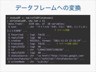
![status
> # R5
> ls.str(statuses[[1]])
created : POSIXct[1:1], format: "2011-11-23 22:16:24"
favorited : logi FALSE ↑ UTC
id : chr "139467359571296256"
initFields : Formal class 'refMethodDef' [package "methods"]
with 5 slots
initialize : Formal class 'refMethodDef' [package "methods"]
with 5 slots
replyToSID : chr(0)
replyToSN : chr(0)
replyToUID : chr(0)
screenName : chr "a_bicky" ! Twitter
statusSource : chr "<a href="http://sites.google.com/site/
yorufukurou/" rel="nofollow">YoruFukurou</a>"
text : chr " "
truncated : logi FALSE ↑](https://image.slidesharecdn.com/twitteranalyticsforslideshare-111126004229-phpapp01/85/R-Twitter-16-320.jpg)
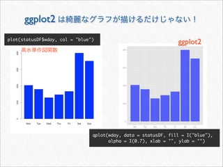
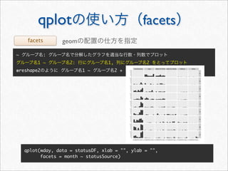
![> # Twitter
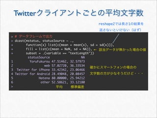
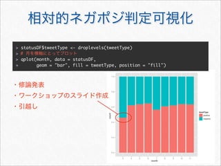
> topSources <- names(head(sort(table(statusDF$statusSource),
decreasing = TRUE), 5))
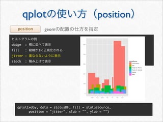
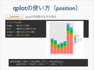
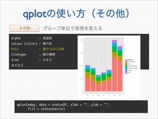
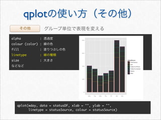
> statusDF <- within(statusDF, {
+ statusSource <- as.character(statusSource)
+ statusSource[!statusSource %in% topSources] <- "other"
+ #
+ statusSource <- factor(statusSource, levels = names(sort(table
(statusSource), dec = TRUE)))
+ })](https://image.slidesharecdn.com/twitteranalyticsforslideshare-111126004229-phpapp01/85/R-Twitter-19-320.jpg)
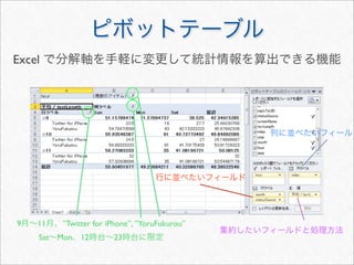
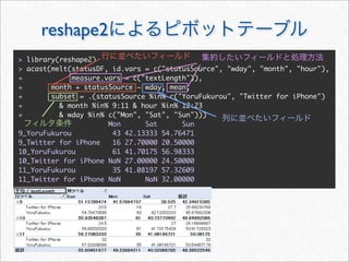
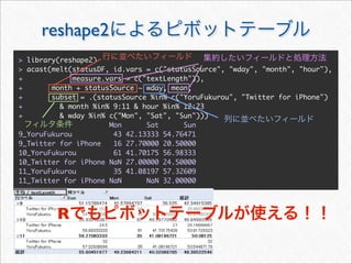
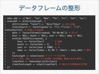
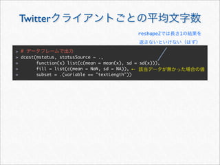
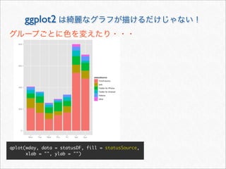
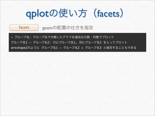
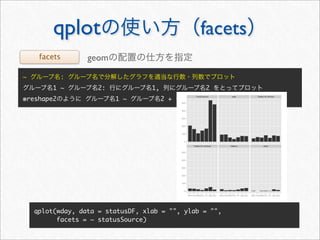
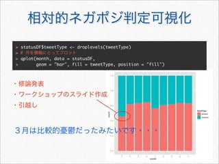
![reshape2 melt
melt cast
melt
cast
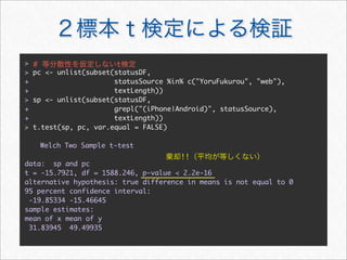
> mstatus <- melt(statusDF,
+ id.vars = c("statusSource", "wday", "year", "month", "hour", "date"),
+ measure.vars = c("textLength", "cleanTextLength"))
> mstatus[3157:3162, ]
statusSource wday year month hour date variable value
3157 web Sun 2011 3 20 2011-03-13 textLength 72
3158 web Sun 2011 3 16 2011-03-13 textLength 24
3159 web Sun 2011 3 14 2011-03-13 textLength 82
3160 YoruFukurou Wed 2011 11 1 2011-11-23 cleanTextLength 87
3161 YoruFukurou Wed 2011 11 1 2011-11-23 cleanTextLength 14
3162 YoruFukurou Wed 2011 11 1 2011-11-23 cleanTextLength 21
id](https://image.slidesharecdn.com/twitteranalyticsforslideshare-111126004229-phpapp01/85/R-Twitter-27-320.jpg)
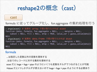
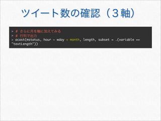
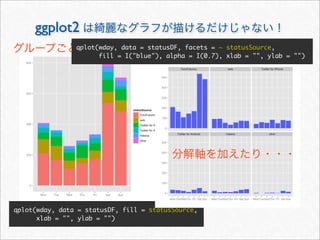
![> #
> acast(mstatus, . ~ wday, length, subset = .(variable == "textLength"))
Mon Tue Wed Thu Fri Sat Sun
[1,] 408 360 258 294 334 801 704
>](https://image.slidesharecdn.com/twitteranalyticsforslideshare-111126004229-phpapp01/85/R-Twitter-30-320.jpg)
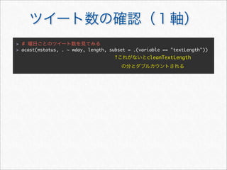
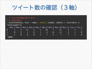
![> #
> acast(mstatus, . ~ wday, length, subset = .(variable == "textLength"))
Mon Tue Wed Thu Fri Sat Sun
[1,] 408 360 258 294 334 801 704
>](https://image.slidesharecdn.com/twitteranalyticsforslideshare-111126004229-phpapp01/85/R-Twitter-31-320.jpg)
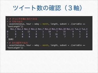
![> #
> acast(mstatus, . ~ wday, length, subset = .(variable == "textLength"))
Mon Tue Wed Thu Fri Sat Sun
[1,] 408 360 258 294 334 801 704
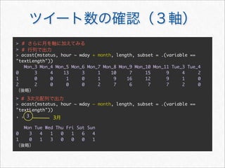
> #
> acast(mstatus, hour ~ wday, length, subset = .(variable ==
"textLength"))](https://image.slidesharecdn.com/twitteranalyticsforslideshare-111126004229-phpapp01/85/R-Twitter-32-320.jpg)
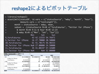
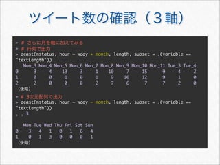
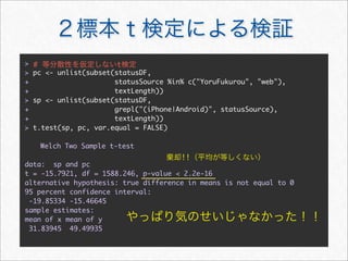
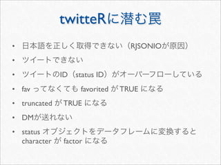
![> #
> acast(mstatus, . ~ wday, length, subset = .(variable == "textLength"))
Mon Tue Wed Thu Fri Sat Sun
[1,] 408 360 258 294 334 801 704
> #
> acast(mstatus, hour ~ wday, length, subset = .(variable ==
"textLength"))
Mon Tue Wed Thu Fri Sat Sun
0 65 69 26 46 46 49 40
1 48 19 11 15 27 44 37
2 31 24 6 16 17 23 17
3 27 19 4 11 14 17 10
4 4 15 1 7 4 5 7
5 5 11 1 4 3 4 5
6 4 14 3 6 9 8 1](https://image.slidesharecdn.com/twitteranalyticsforslideshare-111126004229-phpapp01/85/R-Twitter-33-320.jpg)


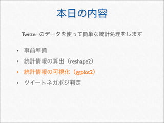
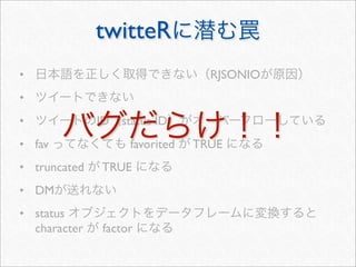
![> extractScreenNames <- function(text, strict = TRUE) {
+ if (strict) {
+ # Twitter screen_name
+ regex <- "(?:(?<!w)([@ ])((?>w+))(?![@ ])|[sS])"
+ } else {
+ # hoge@example.com
+ regex <- "(?:([@ ])(w+)|[sS])"
+ }
+ screenNames <- gsub(regex, "12", text, perl = TRUE)
+ unique(unlist(strsplit(substring(screenNames, 2), "[@ ]")))
+ }
> screenNames <- unlist(lapply(statusDF$text, extractScreenNames))
> head(sort(table(screenNames), decreasing = TRUE), 10) # Top 10
screenNames
naopr __gfx__ hirota_inoue mandy_44 ask_a_lie
105 85 51 47 40
ken_nishi nokuno yokkuns JinJin0613 kanon19_rie
39 39 33 20 20](https://image.slidesharecdn.com/twitteranalyticsforslideshare-111126004229-phpapp01/85/R-Twitter-47-320.jpg)


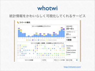
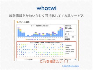
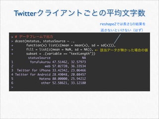
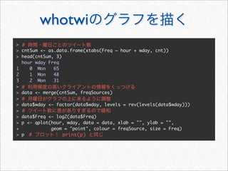
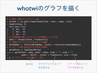
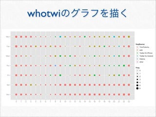
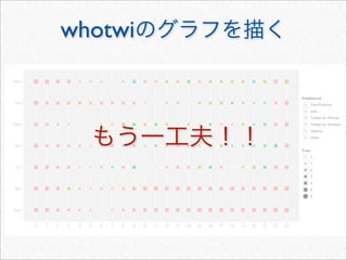
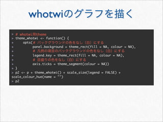
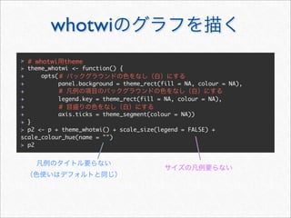
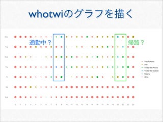
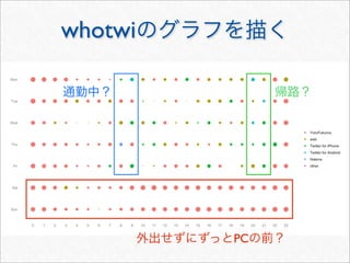
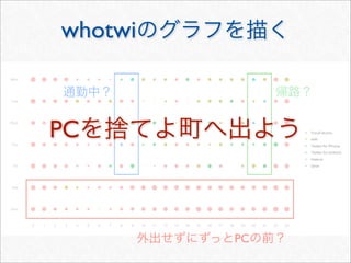
![whotwi
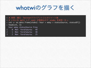
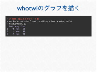
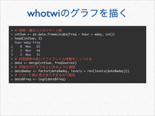
> # Twitter
> # melt cast xtabs
> cnt <- as.data.frame(xtabs(~ hour + wday + statusSource, statusDF))
> head(cnt, 3)
hour wday statusSource Freq
1 0 Mon YoruFukurou 48
2 1 Mon YoruFukurou 38
3 2 Mon YoruFukurou 25
> freqSources <- by(cnt, cnt[c("hour", "wday")], function(df) {
+ #
+ freqSource <- with(df, statusSource[order(Freq, decreasing = TRUE)
[1]])
+ cbind(df[1, c("hour", "wday")], freqSource)
+ })
> freqSources <- do.call(rbind, freqSources)
> head(freqSources, 3)
hour wday freqSource
1 0 Mon YoruFukurou
2 1 Mon YoruFukurou
3 2 Mon YoruFukurou](https://image.slidesharecdn.com/twitteranalyticsforslideshare-111126004229-phpapp01/85/R-Twitter-78-320.jpg)

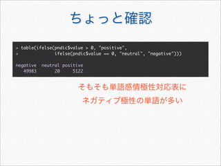
![> # pndic
> pos <- unique(pndic2$pos)
> tweetDF <- docDF(statusDF, column = "cleanText", type = 1, pos = pos)
number of extracted terms = 7164
now making a data frame. wait a while!
> tweetDF[2900:2904, 1:5]
TERM POS1 POS2 Row1 Row2
2900 0 0
2901 0 0
2902 0 0
2903 0 0
2904 0 0
> # pndic
> tweetDF <- subset(tweetDF, TERM %in% pndic2$term)
> #
> tweetDF <- merge(tweetDF, pndic2, by.x = c("TERM", "POS1"), by.y = c
("term", "pos"))](https://image.slidesharecdn.com/twitteranalyticsforslideshare-111126004229-phpapp01/85/R-Twitter-101-320.jpg)
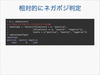
![> #
> score <- colSums(tweetDF[4:(ncol(tweetDF) - 1)] * tweetDF$value)
> #
> sum(score > 0)
[1] 117](https://image.slidesharecdn.com/twitteranalyticsforslideshare-111126004229-phpapp01/85/R-Twitter-102-320.jpg)
![> #
> score <- colSums(tweetDF[4:(ncol(tweetDF) - 1)] * tweetDF$value)
> #
> sum(score > 0)
[1] 117](https://image.slidesharecdn.com/twitteranalyticsforslideshare-111126004229-phpapp01/85/R-Twitter-103-320.jpg)
![> #
> score <- colSums(tweetDF[4:(ncol(tweetDF) - 1)] * tweetDF$value)
> #
> sum(score > 0)
[1] 117
> #
> sum(score < 0)
[1] 2765](https://image.slidesharecdn.com/twitteranalyticsforslideshare-111126004229-phpapp01/85/R-Twitter-104-320.jpg)
![> #
> score <- colSums(tweetDF[4:(ncol(tweetDF) - 1)] * tweetDF$value)
> #
> sum(score > 0)
[1] 117
> #
> sum(score < 0)
[1] 2765](https://image.slidesharecdn.com/twitteranalyticsforslideshare-111126004229-phpapp01/85/R-Twitter-105-320.jpg)
![> #
> score <- colSums(tweetDF[4:(ncol(tweetDF) - 1)] * tweetDF$value)
> #
> sum(score > 0)
[1] 117
> #
> sum(score < 0)
[1] 2765
> #
> sum(score == 0)
[1] 277](https://image.slidesharecdn.com/twitteranalyticsforslideshare-111126004229-phpapp01/85/R-Twitter-106-320.jpg)
![> #
> score <- colSums(tweetDF[4:(ncol(tweetDF) - 1)] * tweetDF$value)
> #
> sum(score > 0)
[1] 117
> #
> sum(score < 0)
[1] 2765
> #
> sum(score == 0)
[1] 277](https://image.slidesharecdn.com/twitteranalyticsforslideshare-111126004229-phpapp01/85/R-Twitter-107-320.jpg)
![> #
> score <- colSums(tweetDF[4:(ncol(tweetDF) - 1)] * tweetDF$value)
> #
> sum(score > 0)
[1] 117
> #
> sum(score < 0)
[1] 2765
> #
> sum(score == 0)
[1] 277](https://image.slidesharecdn.com/twitteranalyticsforslideshare-111126004229-phpapp01/85/R-Twitter-108-320.jpg)


![status
> statuses[[1]]$text
[1] " "
> statuses[[1]]$getText() #
[1] " "
> #
> statuses[[1]]$text <- " "
> statuses[[1]]$getText()
[1] " "
> statuses[[1]]$setText("ggrks") #
> statuses[[1]]$getText()
[1] "ggrks"
> #
> statuses[[1]]$getCreated()
[1] "2011-11-23 22:16:24 UTC"](https://image.slidesharecdn.com/twitteranalyticsforslideshare-111126004229-phpapp01/85/R-Twitter-127-320.jpg)
(?![@ ])"
} else {
regex <- "[@ ]w+"
}
gsub(regex, "", text, perl = TRUE)
}](https://image.slidesharecdn.com/twitteranalyticsforslideshare-111126004229-phpapp01/85/R-Twitter-129-320.jpg)
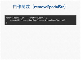
![removeURL
removeURL <- function(text, strict = TRUE) {
if (strict) {
regex <- "(?<![-.w#@=!'"/])https?://(?:[^:]+:.
+@)?(?:[0-9A-Za-z][-0-9A-Za-z]*(?<!-).)+[A-za-z]+(?:/[-
w#%=+,.?!&~]*)*"
} else {
regex <- "https?://[-w#%=+,.?!&~/]+"
}
gsub(regex, "", text, perl = TRUE)
}](https://image.slidesharecdn.com/twitteranalyticsforslideshare-111126004229-phpapp01/85/R-Twitter-130-320.jpg)
![removeHashTag
removeHashTag <- function(text, strict = TRUE) {
delimiters <- "s,.u3000-u3002uFF01uFF1F"
# cf. http://nobu666.com/2011/07/13/914.html
validJa <- "u3041-u3094u3099-u309Cu30A1-u30FA
u30FCu3400-uD7A3uFF10-uFF19uFF21-uFF3AuFF41-uFF5A
uFF66-uFF9E"
if (strict) {
regex <- sprintf("(^|[%s])(?:([# ](?>[0-9]+)(?!
w))|[# ][w%s]+)", delimiters, validJa, validJa)
} else {
regex <- sprintf("[# ][^%s]+", delimiters)
}
gsub(regex, "12", text, perl = TRUE)
}](https://image.slidesharecdn.com/twitteranalyticsforslideshare-111126004229-phpapp01/85/R-Twitter-131-320.jpg)

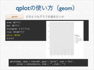
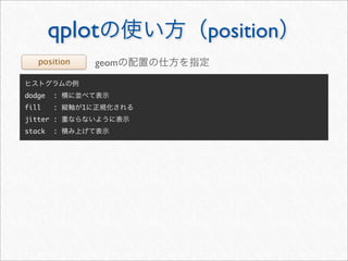
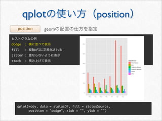
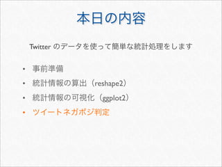
This document discusses analyzing Twitter data from the user @a_bicky using R. It extracts over 3,200 tweets from the user's timeline using the twitteR package. The tweets are transformed into a data frame with variables like text, date, and source. The data is then summarized using the reshape2 and ggplot2 packages to calculate metrics like average text length by day of week, month, and source. Frequency tables and heat maps are generated to explore patterns in the Twitter data over time.