2014-sem2-cven90022-387154-621052

of 39
Dept of Infrastructure Engineering. Research Paper for CVEN90022,
Copyright © Yuchen Cao, Zhao Liu 2014.
Appling cargo bicycles for last kilometer deliveries in
central city areas of Melbourne
Yuchen Cao
The University of Melbourne, Melbourne, Australia
caoyc@student.unimelb.edu.au
Zhao Liu
The University of Melbourne, Melbourne, Australia
zliu3@student.unimelb.edu.au
Abstract:
The increasing population generates more demands of goods deliveries, which brings
successive issues including pollution and congestion in the Melbourne central business
district (CBD). Most of the issues are caused by the traditionally fuel powered vans. Last
kilometre delivery is the most expensive part of the city logistics network as central area
always facing the congestion problem. Cargo bicycles have been considered as
environmental friendly tools that can be used for last kilometre deliveries in central city area
in order to reduce the congestion and pollution leaded by vans. However, bicycles are limited
by the delivery range and capacity, which largely affects its practicability. Therefore, the aim
of this research project is to apply the cargo bicycles for last kilometre deliveries in central
city areas by the establishments of Urban Consolidation Terminals. In this logistic system,
logistics companies drop off their goods to the terminals which are located close to the area
they are served. The goods are sorted and redistributed by the terminal operators and
delivered by the bicycles to the final destinations. The successful city logistic networks
require the optimisation of vehicle routes, schedules and the terminal locations. Therefore,
different models of the city logistics networks will be developed and evaluated by comparing
the total travelled distance, time, emissions and cost. The most effective model of the city
logistic network that applies the cargo bicycle for last kilometre deliveries in Melbourne CBD
will be suggested. This research fills the blanks and brings benefits for Melbourne city
logistic network in terms of the economic, social and environmental aspects.

of 39
1. Introduction:
Goods deliveries play a significant role in people’s daily life. For residents, they provide
sufficient supplies to meet their basic needs. For companies, goods deliveries ensure the
linkages between suppliers and customers are smooth (Crainic, Ricciardi, & Storchi, 2004). In
Melbourne CBD, delivery demands have been increasing rapidly as resident growth which
further contributes to the increase of the numbers of delivery vehicles. The traditional fueled
vans bring about serious issues to urban transport system including congestion and
greenhouse gas emissions.
There are no effective freight solutions to solve such issues in Melbourne. Although
congestion levy has been imposed to CBD area, the quantity of traffic vehicles is still
increasing. In Europe, some cities have applied cargo bicycles for goods deliveries in last
kilometres (urban areas) to the final destinations. Cargo bicycles can effectively reduce the
congestion as they require fewer spaces. They also bring about sufficient environmental
benefits in terms of the reduction on emissions. However, bicycle deliveries are limited by the
delivery distance and goods capacity, which brings out the needs for establishments of Urban
Consolidation Terminals. With the use of the terminals, logistics companies are able to drop
off their goods to the terminals which are located near the city centre; the goods are sorted
and allocated at the terminals. Finally the bicycles are used to deliver the goods to customers.
This paper aims to model the effective city logistic network for Melbourne. Different models
are going to be developed and evaluated by four criteria including total travelled distance,
travel time, emissions and cost. Finally, the optimal model of the city logistic network for
Melbourne is suggested.
2. Literature review
2.1 Current traffic issues in Melbourne CBD
Melbourne currently suffers from traffic congestions and extremely high vehicle volumes in
CBD area. Current urban logistics use vans to deliver goods to customers located within the
CBD, which plays a significant role in the level of congestion. The increasing demands of the
goods deliveries are leaded by the population growth, which makes the congestion worse.
2.1.1 Demand
The growing number of the central city residents and retail stores causes the increasing
demands for freight deliveries associated with fresh food, mail and clothing etc. The census of
land use and employment (CLUE) provides the integrated information about land use,
employment and economic activity across the City of Melbourne. This information gives the
ideas about the distribution and density of the demands. It suggested the number of cafes and
restaurants increased by 12%, and the residential apartments increased by5% from 2008 to
2010. (City of Melbourne, 2015). The increasing demands contribute to congestion in
Melbourne CBD.

of 39
2.1.2 Van-related congestion
Congestion is a serious problem for Melbourne CBD. A survey shows that vans delivery
accounts for 7to 15% of VKM in urban areas and the congestion impacts caused by each van
can be two times that of a passenger vehicle (Russell G, 2013). It is suggested that Melbourne
traffic congestion produces nearly 2.9 million tonnes of carbon dioxide per year (Harris,
2008). Congestion will increase fuel consumption by 30% percent. In addition, noise and
vibration caused by congestion leads to the environmental aesthetic disappearing. The
negative economic effects including reduced productivity of transport and inefficient use of
fuel (Clarke, 2006). There are numerous tools to reduce congestion. One of them is demand-
oriented strategy, which means using delivery consolidation to reduce or shift truck traffic
(Russell G, 2013).
2.2 Last kilometre deliveries
Due to the specific demand, the last kilometre delivery is regarded as the most expensive
sector of the whole logistics network (Maes & Vanelslander, 2012). It is the final step of
goods delivery to the customers who accept the commodities at home or a collection place.
According to a series of research of last kilometre delivery, this part takes 13% to 75% of the
total delivery cost (Muñuzuri, Larrañeta, Onieva, & Cortés, 2005). Moreover, the last
kilometre deliveries are inefficient and they are contributing main source of environment
pollution.
2.3 Cargo bicycles
In Europe, there are growing concerns on using cargo bicycles to decrease the quantities of
traffic vehicles in city areas(Goldman & Gorham, 2006). In London and Berlin, the cargo
bicycle delivery system has already been established by local governments and logistic
companies. Cargo bicycles for goods deliveries provide a good solution to reduce road
congestion, environmental pollution caused by traffic vehicles and parking issues(Crainic,
Ricciardi, & Storchi, 2004). Currently, cargo bicycle deliveries are mainly used for courier
services, including packages, letters and documents. Moreover, the fast food grows quickly
and it also becomes a main part use of bicycle deliveries. A successful case is the bicycle
delivery system established between London and Cambridge. The delivery system is made up
by using folding bikes in urban area and trains between cities(Maes & Vanelslander, 2012). In
addition, another successful case is DHL Netherlands that is a famous global parcel delivery
company. It substituted 33 trucks for 33 cargo bicycles in 15 Dutch cities, which decreased
152 metric tons of carbon dioxides and €430,000 per year(Crainic et al., 2004). However, the
batteries of cargo bicycles cannot be ignored. Cargo bicycles are mainly powered by people
(some types of bicycles have electric power), which limits the delivery distances and goods
weights. The “bikeable” distance is seven kilometres or less, and the heaviest weight per
parcel can only reach 20 to 30 kg averagely(Crainic et al., 2004).
2.4 Urban consolidation terminals
Urban consolidation terminals are also named as urban consolidation centres that are logistics
facilities established to reduce unnecessary vehicle movement, congestion and pollution. The
location of the terminals are situated in particular close proximity to the urban area they are

of 39
served. Europe’s Urban Consolidation Terminals is an attractive option for Melbourne’s city
logistics. In their system, terminal operators sort and redistribute the goods dropped by the
freight logistics companies and then using environmentally friendly vehicles to deliver the
goods to the final destinations (Allen, 2005). Utrecht is the fourth largest city in Netherlands,
it builds a transfer terminal located 300m away from the start of the time window limit zone
of the central city area. All the low-weighted retail goods are delivered to the terminal and use
the electrically powered goods vehicles named Cargohopper to deliver the goods to the final
destinations in central Utrecht. It is estimated that the freight bundling in the city logistic
system undertook 16,500 conventional goods vehicle trips into the city are which equates to
the reduction of 122,000 vehicle-km and 34 tonnes of carbon dioxide (MDS Transmodal,
2012). Integrating the terminals into the city logistics system in order to achieve the full
function of the terminals requires careful model development. The modelling requires
optimization of the vehicle routes, schedules and terminal locations.
2.5. Evaluation criteria
The criteria used to evaluate the city logistics systems are outlined and discussed below.
2.5.1 Total travelled distance
City of Melbourne provides a range of Melbourne CBD traffic network data which includes
the information about the intersections, links and the links distances. The coordinates of the
intersections in Melbourne CBD area are shown in Figure 1.
Figure 1: Coordinates of the intersections in Melbourne CBD (City of Melbourne, 2015)
The total travelled distance needs to be separated into two parts. One is the distance travelling
outside the CBD and the other is the distance travelled within the CBD area.
Distance travelled outside the CBD (supplier to the boundary of the CBD or supplier drops
their certain parcels to the specific terminal). The distance is hard to be calculated accurately,
because streets in suburb areas have many curves and most of them are not straight. Therefore,
Distance vehicle travelled to reach CBD can be calculated by using Equation 1:
𝐷1 = 0.65 × (|𝑋1 − 𝑋2| + |𝑌1 − 𝑌2|)
Where (𝑋1 𝑎𝑛𝑑 𝑌1) are the horizontal and vertical location of the supplier while (𝑋2 𝑎𝑛𝑑 𝑌2) are the location of the
specific point locate at the boundary of the CBD area or the location of the terminals.
The distances travelled within CBD area are calculated by Equation 2:
𝐷2 = (|𝑋 𝐶𝑖+1 − 𝑋 𝐶𝑖| + |𝑌𝐶𝑖+1 − 𝑌𝐶𝑖|)
Where X, Y are the coordinates of customer 𝑖
0
500
1000
1500
0 500 1000 1500 2000 2500
Northing:m
Easting:m
The Melbourne CBD

of 39
The total traveling distance D= 𝐷1 + 𝐷2
Tabu research method is adopted in Equation 2 to derived optimization of vehicle routing
problem (VRP) in order to get shortest distances travelled between the customers and the
terminals.
The Vehicle Routing Problem (VRP) is the problem of finding the optimum routes from the
depots to customers who are distributed in a whole area(Gendreau, Hertz, & Laporte, 1994).
It plays a significant role in logistics. There are many criteria determining the choice of
optimum routes such as minimum total cost. Several metaheuristics have been developed to
solve the VRP, and Tabu Search is one of them. Tabu search is an exploration of the solution
by transferring from a solution xt identified at iteration t to the best solution xt+1 in a subset of
the neighbourhood N(xt) of xt(Cordeau & Laporte, 2005). Because xt+1 may not improve the
solution xt, a Tabu mechanism is used to prohibit the process of repeating a series of solutions.
A simple way can be used to prevent repeats by avoiding the process going back to previous
solutions, but large amounts of bookkeeping are required.
2.5.2 GHG Emissions
GHG emissions are directly related to the energy consumed and the distance travelled by vans.
The energy consumption by vans can be evaluated by Equation 3 (Browne, 2014).
𝐸 = 𝐶 × (
𝐷
100
)
Where 𝐸 is the energy consumption per product unit, C is the average diesel fuel usage of the vehicle
(liters/100km). According to the Australian Bureau of Statistics the average diesel fuel usage of van is 15L/100km.
D is the travelled distance.
Generally, a van uses 50% of the diesel oil and 50% motor gasoline as its fuel in Australia.
The GHG emissions are approximately equal to2.9 kg𝐶𝑂2/𝑙𝑖𝑡𝑟𝑒. Therefore, the amount of
GHG emissions can be calculated by Equation 4 (ECTA, 2011).
𝐸𝑚𝑖𝑠𝑠𝑖𝑜𝑛(𝑘𝑔) = 2.9 × 𝐸
Where E is the energy consumption.
2.5.3 Travel time
Travel time is calculated by the distance travelled divided by the travelling speed.
 For the truck: The travelling speed is 35km/hr outside the CBD area and 20km/hr(fgg)
within the CBD area (Charting Transport, 2013).
 For the bicycle: The travelling speed is 17km/hr (Deakin University, 2015).
2.5.4 Costs
The costs for vans are the sum of the vehicle operational cost (VOC) and the carbon tax.
According to the TransEco Pty Ltd (2013), The VOC of the vans are including labor,
administrations, fuel consumption, tyres, maintenance, capital, insurance and registration. It
suggests VOC is $3.72/km. Dr. Alex (2013) suggests the carbon tax is $24.15/tonne.
𝐶𝑎𝑟𝑏𝑜𝑛 𝑐𝑜𝑠𝑡(𝐴𝑈𝐷) = 0.15 × 𝐷𝑖𝑠𝑡𝑎𝑛𝑐𝑒 ×
24.15
1000
= 0.0105 × 𝐷𝑖𝑠𝑡𝑎𝑛𝑐𝑒

of 39
Therefore the total cost for using vans is equal to
𝑇𝑜𝑡𝑎𝑙 𝑉𝑂𝐶 𝑜𝑓 𝑉𝑎𝑛(𝐴𝑈𝐷) = 3.7305 × 𝐷𝑖𝑠𝑡𝑛𝑐𝑒(𝑘𝑚)
According to the World Road Association PLARC (2012), the operational cost of the bicycle
needs to include the $1/km/parcel and 100 JPY/parcel≈1 AUD /parcel terminal cost.
2.6 Summary
The increasing population in Melbourne CBD leads to the growth of goods delivery
demands, which further requires larger volumes of delivery vehicles. The large numbers
of traffic vehicles bring about the issues of urban road congestion in Melbourne CBD.
Some European cities have applied cargo bicycles into their city logistic networks for
goods deliveries in urban areas as bicycles can solve part of the issues. However, the
limitations of cargo bicycles are also obvious, such as limited travelled distances and goods
weights. In order to apply cargo bicycles to the city logistics system, terminals are needed.
Goods are delivered by vans from depots to terminals and the goods are redistributed at
terminals. Finally, bicycles deliver the sorted goods to customers.
There are normally four criteria considered in evaluating the logistic networks which
including total travelled distance, GHG emissions, travel time, and financial cost.
3. Methodology and method:
3.1 Methodology
The methodologies applied in this project are literature review, data acquisition and model
development.
3.1.1 Literature review.
Literature review helps to gain the basic knowledge about what has been researched by other
people and the methods about how they study similar research projects. In this case, findings
from the literature review will be summarized and used for further analysis, such as key
factors in the city logistics system and the successful experiences on using cargo bicycles for
goods delivery in CBD areas.
3.1.2 Data acquisition.
The feasibility of our research heavily relies on the acquired real data about current city
logistics situation in. Surveys and interviews with the local bicycle delivery company named
Cargone Couriers are conducted to gain the general information on using bicycles for goods
delivery in CBD area and the limitations. Also, the acquired and collected data are used as the
inputs for further analysis.
3.1.3 Model development.
Four integrated models are developed to apply cargo bicycles for the last kilometre delivery
in Melbourne CBD. The most effective model will be chosen by evaluating the key criteria.
The key model development processes will be discussed below (The University of Melbourne,
1999).

of 39
3.2 Method
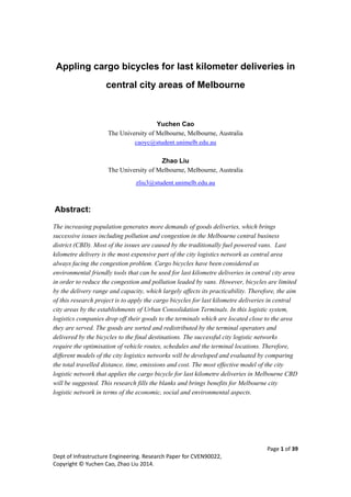
The processes of methods used for the model development are described below and the flow
chart shows the main steps of the methods is shown in Figure 2.
Figure 2: Model development processes (The University of Melbourne, 1999)
Objective
The research method proposed to identify the best structure of the city logistics models that
can apply cargo bicycles for the last kilometre delivery in CBD in Melbourne.
Criteria
 Total travelled distance (which involves the optimization of vehicle routes and schedules
and depot location)
 Environmental impacts (GHG emissions)
 Travel time
 Total cost
System analysis
This process involves identifying the major factors within the system and the relationships
between them. The involved factors are including (Thompson, 2003):
 Supplier locations
 Fleet composition (Vehicle operational cost, speed, emissions..etc)
 Vehicle routes and schedules
 Locations of the terminals
 Demands ( distribution of the customers)
The vehicle routes and schedules and terminals locations are determined by the distribution of
the customers and suppliers. The vehicle operational cost and the amount of emissions are
related with the distance travelled which is directly affected by the vehicle routes and terminal
locations.
System synthesis
This process requires the factors and relationships identified in the system analysis stage to be
represented in the mathematics format by using the variables and the equations to formulate
the model. The equations used are referenced from the literature review part.
Data input
The travel routes in CBD area is measured based on the Melbourne CBD traffic network data,
according to Figure 1.
 Twenty suppliers are randomly chosen outside the analyzed CBD area.

of 39
 Six terminals are evenly located on the boundary of the CBD areas.
 Each supplier has its own set of five customers that are randomly located within the CBD
area, so there are total 100 customers. It is assumed that each customer has one parcel
needs to be delivered.
 Assuming the bicycle only has the capacity to carry 5 parcels at once and each parcel
weighted approximate 1kg.
All data input is shown in Appendix 1.
Software development
Spreadsheet is used to calculate the total travelled distance, travel time, amount of emissions
and cost for each model.
Applications
The concept figure for each model is shown in the Figure 3.
Figure 3: Concept maps of four models
Model 1: Suppliers→customers
Figure 4: Diagram of Model 1
This is the current delivery method that goods are directly delivered by a van from a depot to
5 corresponding customers.

of 39
Model 2: Suppliers → terminals → customers
In this model, each supplier delivers five parcels to a certain terminal by a van. At the
terminal, the staff members transfer the five parcels from the van to a bicycle. The cycle starts
from the terminal and delivers the parcels one by one. After all parcels are delivered, it goes
back to the terminal. All the terminals are tested as one option for each supplier .Tabu search
is applied to find the shortest route travelled by the bicycle from each terminal. The detailed
process of Tabu search is illustrated in Appendix 2. Finally, the travel route chooses for each
supplier is the one with the minimum total financial cost (vans delivery cost plus the bicycle
cost). Therefore the terminal chosen by each supplier will be determined accordingly.
Model 3: Collaborative Distribution. Suppliers→ terminals (bike routes from
terminal𝐬) →Customers
In this case, each supplier drops five parcels by a van to the nearest terminal. The parcels are
reorganized at each terminal and bicycle routes from the terminals are scheduled. For
example, there are two suppliers dropping their parcels at terminal 1 as shown in Figure 6.
Terminal 1 will create two bicycle routes and place 5 parcels in each route according to the
destinations of the parcels to ensure minimum travel distance of each route.

of 39
Model 4. Suppliers→ terminals(𝐓𝐫𝐚𝐧𝐬𝐟𝐞𝐫𝐢𝐧𝐠 𝐩𝐚𝐫𝐜𝐞𝐥𝐬 𝐛𝐞𝐭𝐰𝐞𝐞𝐧 𝐭𝐞𝐫𝐦𝐢𝐧𝐚𝐥𝐬 →bike
routes from terminal𝐬) →Customers
This model achieves the cooperation between the terminals. The CBD area is divided into six
zones according to the locations of the terminals as shown in Figure 7. After suppliers drop
off the parcels to the nearest terminals which is the same as model 3. A joint van will
distribute the parcels to other five terminals according to each parcel’s destination. Finally,
bicycles are used to deliver the parcels from each terminal to the customers. The principle of
creating the bike routes from each terminal is similar to model 3.
4. Results, analysis and findings
The detailed calculations of different criteria for each model including the Tabu research
results are listed in the Appendix. Only summarized results are listed below.
4.1 Travelled Distances
The travelled distances of each model are summarized in table 1.
Table 1: Travelled distances of each model
Distance travelled outside
the CBD by Van (km)
Distance travelled inside the
CBD by Van (km)
Distance travelled inside the
CBD by bicycle(km)
Total travelled
distance(km)
Model 1 33.17 105.84 - 139.01
Model 2 21.77 3.45 115.06 140.28
Model 3 20.5 - 88.77 109.27
Model 4 20.5 7.36 38.38 66.24
Figure 8: Total travelled distances
0
50
100
150
Model 1 Model 2 Model 3 Model 4
Total travelled Distances
Distance travelled inside the CBD by bicycle(km)
Distrance travelled by van (km)

of 39
Total travelled distances are depending on the locations of the suppliers, terminals and
customers. From comparisons, model 4 has the shortest total travelled distances. Model 2 has
similar total travel distances comparing with model 1, which indicates that without the
successful system operation, terminals will not bring too much benefit to the city logistics
network in terms of the travel distances. According to the figure8, it is easily to tell that model
2, 3 and 4 largely decrease the van dependency which brings the solution to the congestion
with the environmental benefits. As each supplier drop off its parcels to the nearest terminal
in model 3 and 4, the distances travelled by the vans outside the CBD are decreased. By
comparing model 2 and 3, the travelling distances within the CBD area reduced by 22.8%
with the collaborative distribution within individual terminals. Model 4 is the most successful
model which reduced 53% of total travel distances comparing with Model 1. The distances
travelled within the CBD by bike are decreased 44.5% by comparing model 4 and model 2
which prove the cooperation between the terminals can effectively minimum the bicycle
travelled distances.
4.2Travel time
Travel time by each model is summarized in table 2.
Table 2: Travel time by each model
Time travelled outside
CBD(mins) by vans
Time travelled inside the
CBD by VAN (mins)
Time travelled inside
the CBD by
bicycle(mins)
Total travel
time(mins)
Model 1 56.86 317.52 - 336.86
Model 2 37.32 10.35 345.18 392.85
Model 3 35.14 - 266.31 348.46
Model 4 35.14 22.08 135.45 192.68
Figure 9: Total travel time of each model
Travel time highly depends on the travel distances of the vehicles and the travel speed of the
vehicles. As mentioned before, the travel speed of the vans outside the CBD is 35km/hr and
the speed within CBD is 20km/hr. bicycles have the travel speed of 17km/hr. Model 3 and 4
prove that if suppliers drop their parcels to the nearest terminals, the travel time will decrease
by 38%. By comparing model 2 and 4, the joint delivery system largely decrease the travel
time within the CBD by 61%. Model 4 achieved approximately 43% overall travel time
savings compare with the Model1. As vans only travel outside and at the boundaries of the
CBD, there are some potential time savings from the congestions alleviation within the CBD
0
200
400
600
Total travel Time(mins)
Total travel Time(mins)

of 39
area. The travel time savings will largely increase the efficiency of the city logistics system
of Melbourne.
4.3 Emissions
The amounts of emissions of each model are summarized in table 3.
Table 3: Amount of emissions of each model
Emissions(kg)
Model 1 60.40
Model 2 10.97
Model 3 8.92
Model 4 9.08
Figure 10: Amount of emissions of each model
From Figure10, it is easy to tell that terminals can effectively reduce the amount of emissions
leads by the van operation. As supplier drops off its parcels to the nearest terminals, model 3
and 4 have less emissions comparing with model 2. Eventhough model 4 has a little bit higher
emissions comparing with model 3 as the use of the low emission vehicles to transfer the
parcels between the terminals, it is acceptable by considering other benefits. Model 4
achieved 85% emission reduction comparing with model 1 which indicates terminals have
dramatic environmental benefits.
4.4 Costs
The costs of each model are listed in Table 4.
Table 4: Costs of each model
Cost(AUD)
Model 1 518.58
Model 2 754.57
Model 3 620.34
Model 4 395.83
0
50
100
Emission(Kg)
Emission(Kg)

of 39
Figure 11: Costs of each model
It is interesting to find that Model2 has the highest financial cost comparing with other 3
models. The main reason is the operational costs of the terminals which including the high
land costs and labor costs. Thus it again proves that the optimization of vehicle routes and
schedules and depot locations plays critical roles in the success of the urban freight system.
Model 4 saves 24% cost comparing with model 1. It is believed that, with the increasing
demand and further investigation of the model, the economic savings will be more enormous.
4.5 Summary of the analysis and findings
From the results, the benefits of applying cargo bicycles to the last kilometre deliveries to the
central business area include:
 Shorter total travel distances. Model 4 successfully achieved 53% saving in distance
travelled which proves that the transferring the parcels between the terminals can
effectively shorter total travel distances.
 Travel time savings .Model 4 saves 43% travel time comparing with the traditional
delivery method which will largely increase the efficiency of the city logistics system of
Melbourne. The decreased number of vans travelled in CBD will leads to congestion
alleviation and brings potential time savings
 Environmental benefits .Model 4 achieved 85% emission reduction as the use of bicycles.
Energy conservation as less vans usage.
 Total cost savings. Model 4 saves 24% cost comparing with the traditional method.
Further investigations need to be conducted to achieve more financial savings
 Traffic removed from CBD. Except mode 1, the other three models largely reduced the
vans dependency to deliver the parcels. The traffic removed from CBD largely increased
urban amenity which brings lots of social benefits.
5. Discussions
5.1 Process and timeline
There are two major parts in our research:
 Literature reviews. Literature reviews are conducted in order to gain the basic knowledge
about the key factors in the city logistics system and the current issues of the logistic
issues in Melbourne.
0
500
1000
Cost(AUD)
Cost(AUD)

of 39
 Model development. Four models are built for comparisons in order to find the best
structure for the city logistics network for Melbourne.
During the first semester of our research, most effort was put on case studies on cities that
have applied cargo bicycles. Generally, those cities such as Amsterdam pay more attention on
their environment and try to minimize the problem of GHG emission and road congestion.
However, their city logistic networks are similar to Model 2 which has the highest cost, and
this is the main reason why terminals haven’t been established in Melbourne. We realised that
the high costs are leaded by long travel distance. And then, we started to seek other
appropriate models in order to minimise the travel distance by freight bundling.
Stage 2 is model development. We started to build our model from the January of 2015. At
first, Genetic Algorithms (GA) was regarded as the optimum method to solve the vehicle
routing problem (VRP). We spent 2 months to study GA in Matlab, but after the study, we
found the GA method was even more complicated than calculating manually. And at that time,
there was only one month before the due day. Thanks to our supervisor, he suggested us to try
Tabu search, and finally it worked. This mistake reminds us a trail is needed for each method.
It is quite time consuming that you study a method well, but finally it is not appropriate for
your research. The result shows that our models match our expectations well, but due to the
limited time, there are many limitations of our research and further research is needed to
make city logistics network more practical and feasible in Melbourne.
5.2 Strengths and limitations
5.2.1 Strengths:
 Feasible and reliable models. Logistics is a complicated problem that includes multiple
suppliers and customers and routes. To make our models more reliable, the process of
modeling was conducted step by step. Firstly, a simple model was built with 1 supplier
and 1 customer to analyse the route between them. Secondly, a more complicated model
was built with 1 supplier serving 5 customers. Finally, the models applied in our research
were built with multiply suppliers and customers. Models were modified continually
during the modelling stage, and the process from simplicity to complication is a good way
to verify the reliability and feasibility.
 Our research is theoretically successful. The results of our research are reasonable and
can match our expectations very well. Model 4 provides a good solution for solving the
issues (e.g., road congestion and high emissions), and the total travelled distance, cost and
time can be reduced dramatically by freight bundling and the cooperation distributions
between the terminals.
 The data used in our research is relatively accurate. Some general information on using
bicycles for goods delivery is obtained from a local cargo company called Cargone
Couriers in Melbourne. In addition, the company’s suggestions were taken for terminal
establishment. Moreover, the map published by the City of Melbourne was used to
measure the travelled distance in Melbourne CBD area, which ensured the reliability of
data.

of 39
5.2.2 Limitations:
 Tabu research. Tabu research is an effective method for solving VRP. However, there is
no guarantee that this method can find the exact solution.
 Terminals are not verified. The locations of terminals are selected based on the map of
Melbourne CBD, the feasibility and these locations are not checked on site. Besides
locations, the fee (1 AUD/parcel) charged in terminals is estimated by a real case in Japan.
However, because the charging fee heavily depends on the land price and labor cost, this
data is not accurate for Melbourne.
 In our study, locations of customers are assumed distributed uniformly in the whole CBD
area. In reality, the customer density is higher in outer CBD and lower in inner CBD area.
This factor was ignored in our research for simplifying models.
5.2.3 Further research
 Applying CLUE data into the research to make the customer distribution closer to the real
situation in the Melbourne CBD.
 Verifying the feasibility of terminals. Many factors can affect the choice of terminals，
including the land price, storage capacity and convenience. Further work needs to
consider all of these factors into terminal establishment.
 Considering more variable goods weight and types. In our research, we assume the
delivery goods are small and light. Further research need to be conducted by considering
more goods types and weights in order to gain more realistic price mechanism.
 Investigations on bike types. The capacity and volume are different between bicycles. The
choice of bicycles might need to be changed according to the goods types and weights.
 Studying intelligent Access Program (IAP) for better road freight management, such as
using GPS to monitor road conditions and heavy vehicles.
 Sensitivity analysis can be made to measure each factor’s degree of influence, such as
labor cost and bike speed.
 Model validation. This process is to test whether the applied models work with the reality.
In our research, many data are assumed without checking real situations, such as terminal
locations and costs. Further studies (e.g., surveys and interviews) are required to check
the rationality of data and models.
6. Conclusions
This research project mainly focuses on developing the effective city logistics network that
apply cargo bicycles for last kilometer deliveries in Melbourne CBD. By comparing four
models developed for the Melbourne CBD city logistic network. The most effective model
with the optimizations of the vehicle routes and schedules and the terminal locations brings
lots of benefits comparing with the current delivery network. In this model, suppliers drop off
their goods to the nearest terminals ensure the minimum traveled distances by vans.
Transferring the goods between the terminals ensure the customers are severed with the
terminals are in close proximity to them. The distances traveled within the CBD are
minimized by using Tabu search. Therefore, the proposed model for city logistic network

of 39
effectively achieves the freight bundling at the terminals, and it achieves 53% saving in
distances traveled. The shorter total travelled distances directly lead to the savings of 43%
travel times and the 24% cost. The use of cargo bicycles for the last kilometer delivery brings
lots of environmental benefits including 85% emission reduction. Moreover, conventional
vans removed from CBD release noise and pollution caused by congestions and increased the
urban amenity. Overall, the proposed model can brings sufficient benefits in terms of the
economic, environmental and social aspects.
However, the real city logistics network is far more complicated than the model has been
developed. Further research need to be conducted to ensure more efficient city logistics
network including more accurate demand estimation, goods types, verification on the
feasibility of the terminals, vehicle types, sensitivity analysis and validation of the model.
References
Alex.R. (2013). Australia’s Carbon Tax. Retrieved from http://instituteforenergyresearch.org/wp-
content/uploads/2013/09/IER_AustraliaCarbonTaxStudy.pdf
Allen, J. (2005). Urban Freight Consolidation Centres. Retrieved from
http://www.researchgate.net/profile/Allan_Woodburn/publication/228761468_Urban_Freight
_Consolidation_Centres_Final_Report/links/00b49529f5794a4973000000.pdf
Browne, M. (2014). Increase urban freight efficiency with delivery and servicing plan. Retrieved from
http://www.researchgate.net/profile/Paulus_Aditjandra/publication/267628526_Increase_urba
n_freight_efficiency_with_delivery_and_servicing_plan/links/5465190a0cf2f5eb17ff3679.pdf
Charting Transport. (2013). Trends in Melbourne Traffic | Charting Transport on WordPress.com.
Charting Transport. Retrieved May 29, 2015, from
http://chartingtransport.com/2010/10/31/trends-in-melbourne-traffic/
City of Melbourne. (2015, February). Census of Land Use and Employment (CLUE). Retrieved from
https://www.melbourne.vic.gov.au/AboutMelbourne/Statistics/CityEconomy/Pages/CLUE.asp
x
Clarke, H. (2006). Economic Framework for Melbourne. Retrieved from http://press.anu.edu.au/wp-
content/uploads/2011/06/13-1-a-5.pdf
Cordeau, J. F., & Laporte, G. (2005). Tabu search heuristics for the vehicle routing problem.
Metaheuristic Optimization via Memory and Evolution. doi:10.1007/BF02579017
Crainic, T. G., Ricciardi, N., & Storchi, G. (2004). Advanced freight transportation systems for
congested urban areas. Transportation Research Part C: Emerging Technologies, 12(2), 119–
137. doi:10.1016/j.trc.2004.07.002
Deakin University. (2015). Walking and cycling to Deakin. Deakin University. Retrieved May 29,
2015, from http://www.deakin.edu.au/life-at-deakin/get-to-deakin/walking-and-cycling-to-
deakin

of 39
ECTA. (2011). Guidelines for Measuring and Managing CO2. Retrieved from
http://www.cefic.org/Documents/IndustrySupport/Transport-and-
Logistics/Best%20Practice%20Guidelines%20-%20General%20Guidelines/Cefic-
ECTA%20Guidelines%20for%20measuring%20and%20managing%20CO2%20emissions%2
0from%20transport%20operations%20Final%2030.03.201
Gendreau, M., Hertz, a., & Laporte, G. (1994). A Tabu Search Heuristic for the Vehicle Routing
Problem. Management Science, 40(10), 1276–1290. doi:10.1287/mnsc.40.10.1276
Goldman, T., & Gorham, R. (2006). Sustainable urban transport: Four innovative directions.
Technology in Society, 28(1-2), 261–273. doi:10.1016/j.techsoc.2005.10.007
Harris, M. (2008). On the Road to greener motoring. Retrieved from http://www.aaa.asn.au/storage/1-
AAA%20Climate%20Change%20Statement%202008.pdf
Maes, J., & Vanelslander, T. (2012). The Use of Bicycle Messengers in the Logistics Chain, Concepts
Further Revised. Procedia - Social and Behavioral Sciences, 39(5), 409–423.
doi:10.1016/j.sbspro.2012.03.118
MDS Transmodal. (2012, April). European Commission:Study on Urban freight transport. Retrieved
from http://ec.europa.eu/transport/themes/urban/studies/doc/2012-04-urban-freight-
transport.pdf
Muñuzuri, J., Larrañeta, J., Onieva, L., & Cortés, P. (2005). Solutions applicable by local
administrations for urban logistics improvement. Cities, 22(1), 15–28.
doi:10.1016/j.cities.2004.10.003
PLARC. (2012). Public sector governance of urban freight transport. Retrieved from
http://www.ite.org.au/public/editor_images/2014%20ITE%20Seminar%20-
%20Russell%20Thompson.pdf
Russell G, T. (2013). City Logistics: Mapping The Future.
The University of Melbourne. (1999). Introduction to Engirnnering systems management, the model
development process.
TransEco Pty Ltd. (2013). TransEco Road Freight Cost Indices (TRFCI). Retrieved from
http://www.transecopl.com/index.php?option=com_content&view=category&layout=blog&id
=4&Itemid=5

of 39
Appendix
Appendix 1
Figure 12: Coordinates of all suppliers, terminals and customers
-2000
-1000
0
1000
2000
3000
4000
-900 100 1100 2100 3100
Northing/m
Easting/m
Locations of suppliers customers and termianls
Suppliers
Customers
Terminals

of 39
Appendix 2 Processes of Tabu Search
Table 5: Distances between customers and terminal
T1 1 2 3 4 5
0 0.920 2.875 1.610 1.725 0.920
1 1.955 0.690 0.345 0.460
2 - 1.265 1.150 1.955
3 - 1.035 1.150
4 - 0.805
5 -
0 represents a terminal and 1,2,3,4 and 5 represent each customer. The distances between
each customer, and the distances between the terminal and each customer are listed in Table 1.
Table 6: 15 Routes of bicycle delivery
Position 1 2 3 4 5 1  
Initial Solutions total distance
Swap Position 0 4 5 2 1 3 0 8.74 R NO.1
( 1 , 2 ) 0 5 4 2 1 3 0 -0.81 -0.81 -1.61 7.13 R NO.2
( 2 , 3 ) 0 4 2 5 1 3 0 0.35 -1.50 -1.15 7.59 R NO.3
( 3 , 4 ) 0 4 5 1 2 3 0 -1.50 0.58 -0.92 7.82 R NO.4
( 4 , 5 ) 0 4 5 2 3 1 0 -0.69 -0.69 -1.38 7.36 R NO.5
The second Solutions
( 1 , 2 ) 0 3 1 5 2 4 0 0.69 -0.69 0.00 7.59 R NO.7
( 2 , 3 ) 0 1 5 3 2 4 0 -0.23 -0.69 -0.92 6.67 R NO.8
( 3 , 4 ) 0 1 3 2 5 4 0 0.12 -0.35 -0.23 7.36 R NO.9
( 4 , 5 ) 0 1 3 5 4 2 0 -1.15 1.15 0.00 7.59 R NO.10
The third solutions
( 1 , 2 ) 0 2 5 3 4 1 0 1.96 -0.12 1.84 8.28 R NO.12
( 2 , 3 ) 0 5 3 2 4 1 0 -0.81 0.12 -0.69 5.75 R NO.13
( 3 , 4 ) 0 5 2 4 3 1 0 -0.12 0.35 0.23 6.67 R NO.14
( 4 , 5 ) 0 5 2 3 1 4 0 -0.35 0.81 0.46 6.90 R NO.15

of 39
Step 1. Picking up a route randomly and each distance can be read from Table 1. As shown in
Table 2, the Route No.1 is from the terminal to Customer 4, then to Customer 5, Customer 2,
Customer 1, Customer 3, and finally back to the terminal. The total distance for Route No.1 is
8.7 km.
Step 2. Swapping the two adjacent positions to generate a new route No.2. Changing the first
and second positions, which means the order of Customer 5 and Customer 4 is swapped. And
then, we get the Route No.2. the Route No.3 can be got by swapping the second and third
positions. The route No.4 and No.5 are got by the same method. These 5 routes are called as
initial solutions.
Step 3.The second solutions start from choosing a new route that is different from the 5 routes
in the first generation. And then, producing the left 4 routes by the same method.
Step 4. Producing the third solutions.
Step 5. There are total 15 routes, and selecting the route with the shortest distance as the
bicycle travelled distance.

of 39
Appendix 3
Table 7: Model 1
supplier
outsider
CBD(m)
Time
travelled
outside
CBD(mins)
In
CBD(m)
Time travelled
inside CBD(mins)
total
distance
Total
travel
time
total
cost
Fuel
consumpti
on (L)
Emissio
ns (kg)
total travel
system cost
1 2.11 1.23 5.75 17.25 7.86 18.48 29.31 1.18 3.42 518.58
2 3.53 2.06 5.06 15.18 8.59 17.24 32.03 1.29 3.74
3 2.93 1.71 5.29 15.87 8.22 17.58 30.67 1.23 3.58
4 1.74 1.02 4.60 13.80 6.34 14.82 23.66 0.95 2.76
5 1.44 0.84 4.72 14.15 6.16 14.99 22.97 0.92 2.68
6 1.22 0.71 4.14 12.42 5.36 13.13 19.99 0.80 2.33
7 1.18 0.69 5.29 15.87 6.47 16.56 24.15 0.97 2.82
8 1.14 0.67 5.75 17.25 6.89 17.92 25.72 1.03 3.00
9 1.62 0.94 4.14 12.42 5.76 13.36 21.48 0.86 2.50
10 3.25 1.90 5.64 16.91 8.89 18.80 33.16 1.33 3.87
11 1.52 0.88 5.52 16.56 7.04 17.44 26.25 1.06 3.06
12 1.69 0.99 4.82 14.46 6.51 15.45 24.30 0.98 2.83
13 1.21 0.71 5.98 17.94 7.19 18.65 26.83 1.08 3.13
14 1.60 0.93 5.61 16.84 7.21 17.77 26.90 1.08 3.14
15 2.10 1.22 5.98 17.94 8.08 19.16 30.14 1.21 3.51

of 39
16 1.62 0.94 5.52 16.56 7.14 17.50 26.63 1.07 3.11
17 0.58 0.34 5.29 15.87 5.87 16.21 21.88 0.88 2.55
18 1.50 0.87 4.60 13.80 6.10 14.67 22.74 0.91 2.65
19 0.70 0.41 6.85 20.56 7.56 20.97 28.19 1.13 3.29
20 0.49 0.29 5.29 15.87 5.78 16.16 21.58 0.87 2.52
139.01 336.86 518.58 20.85 60.47

of 39
Appendix 4:
Table 8: Model 2
su
pp
li
er
te
rn
im
al
out
ter
(km
)
inn
er(
km)
total
truck
distance
(km)
Truck
travelled
time(mins
)
Fuel
consump
tions(L
)
Emis
sion
s(kg
)
total
truck
cost
bike
travel
distanc
e
Bike
travel
led
time
Total
travel
distanc
es
Total
travel
time
total
bike
cost
tot
al
cos
t
opti
mum
cost
total
system
cost
1 1
1.5
0
0.0
0 1.50 2.57 0.23 0.65 5.60 5.75 20.29 7.25 22.87 33.75
39.
35 754.57
2
1.5
0
0.0
0 1.50 2.57 0.23 0.65 5.60 6.21 21.92 7.71 24.49 36.05
41.
65
3
2.5
5
0.0
0 2.55 4.37 0.38 1.11 9.51 6.21 21.92 8.76 26.29 36.05
45.
56
4
2.0
4
1.2
7 3.30 7.29 0.50 1.44 12.33 6.95 24.52 10.25 31.81 39.73
52.
06
5
1.6
5
1.3
8 3.03 6.97 0.45 1.32 11.31 6.44 22.73 9.47 29.70 37.20
48.
51
6
1.5
0
0.9
2 2.42 5.33 0.36 1.05 9.03 6.21 21.92 8.63 27.25 36.05
45.
08
39.3
5
2
1
2.3
6
0.0
0 2.36 4.05 0.35 1.03 8.81 5.98 21.11 8.34 25.15 34.90
43.
71
2
1.9
4
0.0
0 1.94 3.33 0.29 0.84 7.24 5.52 19.48 7.46 22.81 32.60
39.
84

of 39
3
2.9
9
0.0
0 2.99 5.12 0.45 1.30 11.15 6.67 23.54 9.66 28.66 38.35
49.
50
4
2.4
8
1.2
7 3.74 8.05 0.56 1.63 13.97 6.03 21.27 9.77 29.31 35.13
49.
10
5
2.0
9
1.3
8 3.47 7.72 0.52 1.51 12.95 5.06 17.86 8.53 25.58 30.30
43.
25
6
2.3
6
0.9
2 3.28 6.81 0.49 1.43 12.24 5.52 19.48 8.80 26.29 32.60
44.
84
39.8
4
3
1
2.2
1
0.0
0 2.21 3.79 0.33 0.96 8.26 6.44 22.73 8.65 26.52 37.20
45.
46
2
1.3
7
0.0
0 1.37 2.36 0.21 0.60 5.13 5.52 19.48 6.89 21.84 32.60
37.
73
3
2.4
2
0.0
0 2.42 4.15 0.36 1.05 9.03 6.67 23.54 9.09 27.69 38.35
47.
38
4
1.9
1
1.2
7 3.18 7.07 0.48 1.38 11.86 6.03 21.27 9.20 28.34 35.13
46.
99
5
1.5
2
1.3
8 2.90 6.75 0.44 1.26 10.83 5.29 18.67 8.19 25.42 31.45
42.
28
6
2.2
1
0.9
2 3.13 6.55 0.47 1.36 11.69 6.67 23.54 9.80 30.10 38.35
50.
04
37.7
3
4
1 1.7 0.0 1.77 3.03 0.27 0.77 6.60 5.29 18.67 7.06 21.70 31.45 38.

of 39
7 0 05
2
0.8
7
0.0
0 0.87 1.49 0.13 0.38 3.25 4.83 17.05 5.70 18.54 29.15
32.
40
3
1.5
7
0.0
0 1.57 2.69 0.23 0.68 5.84 5.29 18.67 6.86 21.36 31.45
37.
29
4
1.0
6
1.2
7 2.32 5.61 0.35 1.01 8.67 5.11 18.02 7.43 23.63 30.53
39.
20
5
0.7
2
1.3
8 2.10 5.38 0.32 0.91 7.84 4.60 16.24 6.70 21.61 28.00
35.
84
6
1.7
7
0.9
2 2.69 5.79 0.40 1.17 10.03 6.44 22.73 9.13 28.52 37.20
47.
23
32.4
0
5
1
1.9
2
0.0
0 1.92 3.29 0.29 0.83 7.15 5.87 20.70 7.78 23.99 34.33
41.
48
2
1.0
2
0.0
0 1.02 1.75 0.15 0.44 3.81 5.41 19.08 6.43 20.83 32.03
35.
83
3
1.2
9
0.0
0 1.29 2.21 0.19 0.56 4.80 5.87 20.70 7.15 22.91 34.33
39.
13
4
0.7
8
1.2
7 2.04 5.13 0.31 0.89 7.62 5.87 20.70 7.91 25.83 34.33
41.
95
5
0.8
7
1.3
8 2.25 5.63 0.34 0.98 8.40 4.72 16.64 6.97 22.27 28.58
36.
97
6 1.9 0.9 2.84 6.05 0.43 1.23 10.59 4.72 16.64 7.55 22.69 28.58 39. 35.8

of 39
2 2 16 3
6
1
1.8
9
0.0
0 1.89 3.25 0.28 0.82 7.07 7.13 25.16 9.02 28.41 40.65
47.
72
2
1.0
0
0.0
0 1.00 1.71 0.15 0.43 3.72 5.52 19.48 6.52 21.19 32.60
36.
32
3
0.8
5
0.0
0 0.85 1.47 0.13 0.37 3.19 4.83 17.05 5.68 18.51 29.15
32.
34
4
0.6
1
1.2
7 1.87 4.84 0.28 0.82 6.99 4.37 15.42 6.24 20.26 26.85
33.
84
5
0.8
5
1.3
8 2.23 5.59 0.33 0.97 8.31 4.14 14.61 6.37 20.21 25.70
34.
01
6
1.8
9
0.9
2 2.81 6.01 0.42 1.22 10.50 5.98 21.11 8.79 27.11 34.90
45.
40
32.3
4
7
1
1.9
8
0.0
0 1.98 3.40 0.30 0.86 7.40 6.44 22.73 8.42 26.13 37.20
44.
60
2
1.0
9
0.0
0 1.09 1.86 0.16 0.47 4.05 6.44 22.73 7.53 24.59 37.20
41.
25
3
0.6
4
0.0
0 0.64 1.09 0.10 0.28 2.38 6.90 24.35 7.54 25.44 39.50
41.
88
4
0.7
0
1.2
7 1.96 4.99 0.29 0.85 7.32 6.03 21.27 7.99 26.26 35.13
42.
45

of 39
5
0.9
4
1.3
8 2.32 5.74 0.35 1.01 8.64 5.29 18.67 7.61 24.42 31.45
40.
09
6
1.9
8
0.9
2 2.90 6.16 0.44 1.26 10.83 5.75 20.29 8.65 26.45 33.75
44.
58
40.0
9
8
1
0.7
2
1.8
4 2.56 6.76 0.38 1.11 9.56 6.21 21.92 8.77 28.67 36.05
45.
61
2
1.0
2
0.0
0 1.02 1.75 0.15 0.44 3.81 7.13 25.16 8.15 26.91 40.65
44.
46
3
0.1
2
0.0
0 0.12 0.20 0.02 0.05 0.44 6.44 22.73 6.56 22.93 37.20
37.
64
4
1.5
2
1.2
7 2.78 6.40 0.42 1.21 10.39 6.90 24.35 9.68 30.75 39.50
49.
89
5
1.8
3
1.3
8 3.21 7.28 0.48 1.40 11.99 6.90 24.35 10.11 31.64 39.50
51.
49
6
1.9
2
0.9
2 2.84 6.05 0.43 1.23 10.59 5.75 20.29 8.59 26.34 33.75
44.
34
37.6
4
9
1
1.2
5
1.3
8 2.63 6.28 0.39 1.14 9.80 4.60 16.24 7.23 22.51 28.00
37.
80
2
0.5
0
1.6
1 2.11 5.69 0.32 0.92 7.87 4.14 14.61 6.25 20.30 25.70
33.
57
3 0.4 1.6 2.07 5.62 0.31 0.90 7.74 5.75 20.29 7.82 25.92 33.75 41.

of 39
6 1 49
4
0.4
6
0.0
0 0.46 0.79 0.07 0.20 1.73 5.57 19.64 6.03 20.44 32.83
34.
56
5
0.5
0
0.0
0 0.50 0.86 0.08 0.22 1.87 4.60 16.24 5.10 17.09 28.00
29.
87
6
1.5
5
0.0
0 1.55 2.65 0.23 0.67 5.77 4.60 16.24 6.15 18.89 28.00
33.
77
29.8
7
10
1
3.0
6
0.9
2 3.98 8.01 0.60 1.73 14.85 6.10 21.51 10.08 29.52 35.48
50.
33
2
2.3
1
1.1
5 3.46 7.42 0.52 1.51 12.92 5.64 19.89 9.10 27.31 33.18
46.
10
3
1.5
1
0.7
8 2.29 4.93 0.34 1.00 8.54 7.71 27.19 9.99 32.12 43.53
52.
06
4
1.7
0
0.0
0 1.70 2.92 0.26 0.74 6.35 7.61 26.87 9.31 29.79 43.07
49.
41
5
2.0
2
0.0
0 2.02 3.45 0.30 0.88 7.52 6.90 24.35 8.92 27.81 39.50
47.
02
6
3.0
6
0.0
0 3.06 5.25 0.46 1.33 11.42 6.90 24.35 9.96 29.60 39.50
50.
92
46.1
0
11
1
2.1
9
0.9
2 3.11 6.52 0.47 1.35 11.62 6.90 24.35 10.01 30.87 39.50
51.
12

of 39
2
1.1
5
1.6
1 2.76 6.80 0.41 1.20 10.29 6.21 21.92 8.97 28.71 36.05
46.
34
3
0.6
4
1.2
7 1.90 4.89 0.29 0.83 7.10 6.44 22.73 8.34 27.62 37.20
44.
30
4
0.8
3
0.0
0 0.83 1.43 0.12 0.36 3.11 5.57 19.64 6.40 21.07 32.83
35.
94
5
1.1
5
0.0
0 1.15 1.97 0.17 0.50 4.28 5.52 19.48 6.67 21.45 32.60
36.
88
6
2.1
9
0.0
0 2.19 3.76 0.33 0.95 8.18 5.98 21.11 8.17 24.87 34.90
43.
08
35.9
4
12 1
2.2
1
0.9
2 3.13 6.54 0.47 1.36 11.66 5.52 19.48 8.65 26.03 32.60
44.
26
2
1.1
6
1.1
5 2.31 5.44 0.35 1.00 8.62 4.82 17.02 7.13 22.45 29.11
37.
72
3
0.6
5
1.2
7 1.92 4.91 0.29 0.83 7.15 6.20 21.89 8.12 26.80 36.01
43.
16
4
0.8
5
0.0
0 0.85 1.45 0.13 0.37 3.16 5.79 20.42 6.63 21.88 33.94
37.
09
5
1.1
6
0.0
0 1.16 1.99 0.17 0.50 4.33 5.28 18.64 6.44 20.63 31.41
35.
73
6
2.2
1
0.0
0 2.21 3.78 0.33 0.96 8.23 4.83 17.05 7.04 20.83 29.15
37.
38
35.7
3

of 39
13 1
1.7
3
0.9
2 2.65 5.72 0.40 1.15 9.88 5.98 21.11 8.63 26.83 34.90
44.
78
2
0.6
8
1.1
5 1.83 4.62 0.27 0.80 6.84 6.90 24.35 8.73 28.97 39.50
46.
34
3
0.6
1
1.2
4 1.85 4.77 0.28 0.80 6.90 6.67 23.54 8.52 28.31 38.35
45.
25
4
0.6
1
0.0
0 0.61 1.04 0.09 0.26 2.26 6.26 22.08 6.86 23.12 36.28
38.
54
5
0.6
8
0.0
0 0.68 1.17 0.10 0.30 2.55 6.21 21.92 6.89 23.09 36.05
38.
60
6
1.7
3
0.0
0 1.73 2.96 0.26 0.75 6.45 7.13 25.16 8.86 28.13 40.65
47.
10
38.5
4
14 1
1.5
5
0.9
2 2.47 5.41 0.37 1.07 9.20 6.30 22.24 8.77 27.65 36.51
45.
71
2
0.5
0
1.1
5 1.65 4.31 0.25 0.72 6.16 6.07 21.43 7.72 25.74 35.36
41.
52
3
0.4
6
1.2
4 1.71 4.52 0.26 0.74 6.36 6.07 21.43 7.78 25.95 35.36
41.
72
4
0.4
6
0.0
0 0.46 0.79 0.07 0.20 1.73 6.58 23.22 7.04 24.01 37.89
39.
62
5
0.5
0
0.0
0 0.50 0.86 0.08 0.22 1.87 6.07 21.43 6.57 22.29 35.36
37.
23

of 39
6
1.5
5
0.0
0 1.55 2.65 0.23 0.67 5.77 5.61 19.81 7.16 22.46 33.06
38.
83
37.2
3
15 1
1.6
5
0.9
2 2.57 5.58 0.39 1.12 9.58 5.98 21.11 8.55 26.69 34.90
44.
48
2
1.0
2
1.1
5 2.17 5.21 0.33 0.95 8.11 5.98 21.11 8.15 26.31 34.90
43.
01
3
1.0
2
1.9
6 2.98 7.62 0.45 1.30 11.11 6.90 24.35 9.88 31.97 39.50
50.
61
4
1.3
4
0.0
0 1.34 2.29 0.20 0.58 4.99 6.95 24.52 8.28 26.81 39.73
44.
72
5
1.2
0
0.0
0 1.20 2.06 0.18 0.52 4.47 6.44 22.73 7.64 24.79 37.20
41.
67
6
1.6
5
0.0
0 1.65 2.82 0.25 0.72 6.15 6.21 21.92 7.86 24.74 36.05
42.
20
41.6
7
16 1
0.8
7
1.3
8 2.25 5.63 0.34 0.98 8.40 5.98 21.11 8.23 26.74 34.90
43.
30
2
0.8
8
1.7
3 2.61 6.69 0.39 1.13 9.73 6.21 21.92 8.82 28.61 36.05
45.
78
3
1.1
7
2.4
2 3.59 9.25 0.54 1.56 13.37 7.59 26.79 11.18 36.04 42.95
56.
32
4
1.6
5
0.0
0 1.65 2.82 0.25 0.72 6.14 6.95 24.52 8.59 27.34 39.73
45.
87

of 39
5
1.3
3
0.0
0 1.33 2.28 0.20 0.58 4.97 5.98 21.11 7.31 23.39 34.90
39.
87
6
1.1
7
0.0
0 1.17 2.01 0.18 0.51 4.36 5.52 19.48 6.69 21.49 32.60
36.
96
36.9
6
17 1
0.2
9
0.9
2 1.21 3.25 0.18 0.53 4.51 5.29 18.67 6.50 21.92 31.45
35.
96
2
0.2
9
2.3
0 2.59 7.39 0.39 1.13 9.65 5.41 19.09 8.00 26.49 32.05
41.
70
3
1.7
2
1.2
7 2.99 6.75 0.45 1.30 11.15 5.64 19.91 8.63 26.65 33.20
44.
35
4
1.3
5
0.0
0 1.35 2.31 0.20 0.59 5.03 5.46 19.26 6.81 21.57 32.28
37.
31
5
1.0
4
0.0
0 1.04 1.78 0.16 0.45 3.86 5.41 19.09 6.45 20.87 32.05
35.
91
6
0.2
9
0.0
0 0.29 0.49 0.04 0.13 1.07 6.21 21.92 6.50 22.41 36.05
37.
12
35.9
1
18 1
1.1
2
0.9
2 2.04 4.69 0.31 0.89 7.63 6.61 23.33 8.65 28.02 38.05
45.
68
2
1.1
2
2.3
0 3.42 8.83 0.51 1.49 12.78 5.23 18.46 8.65 27.29 31.15
43.
93
3
2.0
7
1.2
7 3.34 7.35 0.50 1.45 12.45 4.60 16.24 7.94 23.58 28.00
40.
45

of 39
4
2.1
9
0.0
0 2.19 3.75 0.33 0.95 8.15 4.60 16.24 6.79 19.98 28.00
36.
15
5
1.8
7
0.0
0 1.87 3.21 0.28 0.81 6.98 5.52 19.48 7.39 22.69 32.60
39.
58
6
1.1
2
0.0
0 1.12 1.93 0.17 0.49 4.19 7.36 25.98 8.48 27.90 41.80
45.
99
36.1
5
19 1
0.7
5
0.0
0 0.75 1.28 0.11 0.33 2.79 8.51 30.04 9.26 31.32 47.55
50.
34
2
0.7
5
1.3
8 2.13 5.42 0.32 0.93 7.94 7.91 27.92 10.04 33.35 44.56
52.
50
3
0.8
2
2.0
7 2.89 7.62 0.43 1.26 10.79 6.85 24.19 9.75 31.81 39.27
50.
06
4
0.5
0
2.3
4 2.84 7.88 0.43 1.24 10.59 7.82 27.60 10.66 35.48 44.10
54.
69
5
0.5
0
1.6
1 2.11 5.69 0.32 0.92 7.87 8.28 29.22 10.39 34.91 46.40
54.
27
6
0.5
0
0.0
0 0.50 0.86 0.08 0.22 1.87 8.51 30.04 9.01 30.89 47.55
49.
42
49.4
2
20 1
0.2
5
0.0
0 0.25 0.42 0.04 0.11 0.92 5.98 21.11 6.23 21.53 34.90
35.
82
2
0.2
5
1.3
8 1.63 4.56 0.24 0.71 6.07 6.44 22.73 8.07 27.29 37.20
43.
27

of 39
3
0.4
0
2.0
7 2.47 6.89 0.37 1.07 9.20 5.29 18.67 7.76 25.56 31.45
40.
65
4
0.5
0
2.0
7 2.57 7.07 0.39 1.12 9.59 6.21 21.92 8.78 28.99 36.05
45.
64
5
0.6
5
1.6
1 2.26 5.94 0.34 0.98 8.43 7.13 25.16 9.39 31.11 40.65
49.
08
6
0.6
5
0.0
0 0.65 1.11 0.10 0.28 2.42 6.67 23.54 7.32 24.66 38.35
40.
77
35.8
2
10.9
7 140.28 453.78
754.
57

of 39
Appendix 5:
Table 9: Model 3
sup
pli
er
ter
min
al
total
truck
distance(
km)
Truck
travel
time( min
s)
Fuel
comsumpt
ions(L)
Emiss
ions
(Kg)
total
truck
cost
total
bike
distanc
e
Bike
travell
ed time
Total
travel
time
total
travel
distance
total
bike
cost
total
termina
l cost
total
travel
system
cost
1 1 1.502 2.574 0.225 0.653 5.601 2.574 1.502 5.601 620.339
20 1 2.988 5.123 0.448 1.300 11.147 10.580 37.341 42.464 13.568 62.900 74.047
2 2 1.942 3.328 0.291 0.845 7.243 3.328 1.942 7.243
3 2 1.375 2.357 0.206 0.598 5.129 2.357 1.375 5.129
4 2 0.871 1.493 0.131 0.379 3.249 1.493 0.871 3.249
5 2 1.021 1.749 0.153 0.444 3.807 13.340 47.082 48.832 14.361 86.700 90.507
6 3 0.855 1.465 0.128 0.372 3.189 1.465 0.855 3.189
7 3 0.637 1.092 0.096 0.277 2.376 1.092 0.637 2.376
8 3 0.117 0.201 0.018 0.051 0.436 13.455 47.488 47.689 13.572 82.275 82.711
9 4 0.463 0.794 0.070 0.202 1.729 0.794 0.463 1.729
10 4 1.701 2.916 0.255 0.740 6.346 2.916 1.701 6.346
11 4 0.833 1.429 0.125 0.362 3.109 1.429 0.833 3.109
12 4 0.846 1.451 0.127 0.368 3.157 1.451 0.846 3.157
13 4 0.606 1.040 0.091 0.264 2.262 1.040 0.606 2.262
14 4 0.463 0.794 0.070 0.202 1.729 23.966 84.586 85.380 24.429 149.83 151.559

of 39
0
15 5 1.199 2.056 0.180 0.522 4.474 6.440 22.729 24.785 7.639 37.200 41.674
16 6 1.170 2.006 0.176 0.509 4.365 2.006 1.170 4.365
17 6 0.288 0.494 0.043 0.125 1.074 0.494 0.288 1.074
18 6 1.125 1.928 0.169 0.489 4.195 1.928 1.125 4.195
19 6 0.501 0.858 0.075 0.218 1.867 20.990 74.082 74.940 21.491
124.95
0 126.817
Tot
al 8.919 239.227
348.45
6 109.273 620.339

of 39
Appendix 6:
Table 10: Model 4
sup
pli
er
ter
min
al
total
truck
distance(
km)
Truck
travle
time(mins
)
Fuel
comsumpt
ions(L)
Emiss
ions
(Kg)
total
truck
cost
total
bike
distanc
e
Bike
travel
time
Total
travel
distance
Total
travel
time
total
bike
cost
total
termina
l cost
total
travel
system
cost
1 1 1.50 2.57 0.23 0.65 5.60 1.50 2.57 5.60 395.83
20 1 2.99 5.12 0.45 1.30 11.15 9.66 34.09 12.65 39.22 68.30 79.45
2 2 1.94 3.33 0.29 0.84 7.24 1.94 3.33 7.24
3 2 1.37 2.36 0.21 0.60 5.13 1.37 2.36 5.13
4 2 0.87 1.49 0.13 0.38 3.25 0.87 1.49 3.25
5 2 1.02 1.75 0.15 0.44 3.81 4.60 16.24 5.62 17.98 38.00 41.81
6 3 0.85 1.47 0.13 0.37 3.19 0.85 1.47 3.19
7 3 0.64 1.09 0.10 0.28 2.38 0.64 1.09 2.38
8 3 0.12 0.20 0.02 0.05 0.44 5.98 21.11 6.10 21.31 44.90 45.34
9 4 0.46 0.79 0.07 0.20 1.73 0.46 0.79 1.73
10 4 1.70 2.92 0.26 0.74 6.35 1.70 2.92 6.35
11 4 0.83 1.43 0.12 0.36 3.11 0.83 1.43 3.11
12 4 0.85 1.45 0.13 0.37 3.16 0.85 1.45 3.16
13 4 0.61 1.04 0.09 0.26 2.26 0.61 1.04 2.26
14 4 0.46 0.79 0.07 0.20 1.73 6.30 22.24 6.77 23.04 46.51 48.24

of 39
15 5 1.20 2.06 0.18 0.52 4.47 4.89 17.26 6.09 19.31 39.45 43.92
16 6 1.17 2.01 0.18 0.51 4.36 1.17 2.01 4.36
17 6 0.29 0.49 0.04 0.13 1.07 0.29 0.49 1.07
18 6 1.12 1.93 0.17 0.49 4.19 1.12 1.93 4.19
19 6 0.50 0.86 0.08 0.22 1.87 6.95 24.52 7.45 25.37 54.73 56.60
City
Loop 7.36 22.08 1.10 3.20 27.46 7.36 22.08 27.46
Tot
al 12.12 66.24 192.68

of 39
Acknowledgements
We would like to thank for the help of our IE research supervisor, Russell G. Thompson
from the University of Melbourne. Also, Graham A. Moore and Yongping Wei also provide
helpful opinions on our project.

2014-sem2-cven90022-387154-621052

Recommended

Recommended

More Related Content

What's hot

What's hot (19)

Viewers also liked

Viewers also liked (8)

Similar to 2014-sem2-cven90022-387154-621052

Similar to 2014-sem2-cven90022-387154-621052 (20)

2014-sem2-cven90022-387154-621052