SlideShare a Scribd company logo
1 of 25
Download to read offline
Task 3 :-
Implement a Generative Adversarial Network (GAN) using TensorFlow or PyTorch to generate
realistic images of a specific object category (e.g., faces, animals). Train the GAN on a small
dataset and showcase a few generated images.
1. Define the Problem and Gather Data
Identify the object category.
Collect a small dataset.
Load DataSet- (CIFAR-10 or CIFAR-100: Small image datasets with multiple classes, including
animals.)
2 . Import necessary libraries
# Import TensorFlow for deep learning
import tensorflow as tf
from tensorflow.keras import layers, models
# Import PyTorch for deep learning
import torch
import torch.nn as nn
import torch.optim as optim
from torch.utils.data import DataLoader
from torchvision import datasets, transforms
from keras.optimizers import Adam
from keras.models import Sequential
from keras.layers import Dense
from keras.layers import Reshape
from keras.layers import Flatten
from keras.layers import Conv2D
# Additional libraries for data manipulation, visualization, and
evaluation
import numpy as np
import matplotlib.pyplot as plt
3.Preprocess Data
# Bringing in tensorflow
import tensorflow as tf
gpus = tf.config.experimental.list_physical_devices('GPU')
for gpu in gpus:
tf.config.experimental.set_memory_growth(gpu, True)
import tensorflow_datasets as tfds
from matplotlib import pyplot as plt
ds = tfds.load('cifar10', split = 'train')
Downloading and preparing dataset 162.17 MiB (download: 162.17 MiB,
generated: 132.40 MiB, total: 294.58 MiB) to
/root/tensorflow_datasets/cifar10/3.0.2...
{"model_id":"dfb4a5deeb4d462399c40d09b145d42c","version_major":2,"vers
ion_minor":0}
{"model_id":"2faacfe454b54aae93c4ecb3642d9107","version_major":2,"vers
ion_minor":0}
{"model_id":"3e5f8e053ec54e269ed2f16ec1d83acd","version_major":2,"vers
ion_minor":0}
{"model_id":"65f1b099d1b04fbaa0cd9c01ae2de919","version_major":2,"vers
ion_minor":0}
{"model_id":"b75145664bc44ebd826b7c0cf0c1fb8b","version_major":2,"vers
ion_minor":0}
{"model_id":"5e169e5cf386472c848f7749150d090c","version_major":2,"vers
ion_minor":0}
{"model_id":"3ce662d8f5f14acf88be11d9551ee0bd","version_major":2,"vers
ion_minor":0}
{"model_id":"6d0c0d7b797840ee8bd707561eed24f7","version_major":2,"vers
ion_minor":0}
Dataset cifar10 downloaded and prepared to
/root/tensorflow_datasets/cifar10/3.0.2. Subsequent calls will reuse
this data.
ds
<_PrefetchDataset element_spec={'id': TensorSpec(shape=(),
dtype=tf.string, name=None), 'image': TensorSpec(shape=(32, 32, 3),
dtype=tf.uint8, name=None), 'label': TensorSpec(shape=(),
dtype=tf.int64, name=None)}>
type(ds)
tensorflow.python.data.ops.prefetch_op._PrefetchDataset
ds.as_numpy_iterator().next()
{'id': b'train_16399',
'image': array([[[143, 96, 70],
[141, 96, 72],
[135, 93, 72],
...,
[ 96, 37, 19],
[105, 42, 18],
[104, 38, 20]],
[[128, 98, 92],
[146, 118, 112],
[170, 145, 138],
...,
[108, 45, 26],
[112, 44, 24],
[112, 41, 22]],
[[ 93, 69, 75],
[118, 96, 101],
[179, 160, 162],
...,
[128, 68, 47],
[125, 61, 42],
[122, 59, 39]],
...,
[[187, 150, 123],
[184, 148, 123],
[179, 142, 121],
...,
[198, 163, 132],
[201, 166, 135],
[207, 174, 143]],
[[187, 150, 117],
[181, 143, 115],
[175, 136, 113],
...,
[201, 164, 132],
[205, 168, 135],
[207, 171, 139]],
[[195, 161, 126],
[187, 153, 123],
[186, 151, 128],
...,
[212, 177, 147],
[219, 185, 155],
[221, 187, 157]]], dtype=uint8),
'label': 7}
ds.as_numpy_iterator().next().keys()
dict_keys(['id', 'image', 'label'])
(train_images, train_labels), (_,_) =
tf.keras.datasets.cifar100.load_data()
print(train_images.shape)
(50000, 32, 32, 3)
train_images = train_images.reshape((50000, 32, 32,
3)).astype('float32')
train_images = (train_images - 127.5) / 127.5 # normalize the images
to [-1,1]
len(train_images)
50000
Data and Build Dataset
import numpy as np
dataiterator = ds.as_numpy_iterator()
dataiterator.next()
{'id': b'train_16399',
'image': array([[[143, 96, 70],
[141, 96, 72],
[135, 93, 72],
...,
[ 96, 37, 19],
[105, 42, 18],
[104, 38, 20]],
[[128, 98, 92],
[146, 118, 112],
[170, 145, 138],
...,
[108, 45, 26],
[112, 44, 24],
[112, 41, 22]],
[[ 93, 69, 75],
[118, 96, 101],
[179, 160, 162],
...,
[128, 68, 47],
[125, 61, 42],
[122, 59, 39]],
...,
[[187, 150, 123],
[184, 148, 123],
[179, 142, 121],
...,
[198, 163, 132],
[201, 166, 135],
[207, 174, 143]],
[[187, 150, 117],
[181, 143, 115],
[175, 136, 113],
...,
[201, 164, 132],
[205, 168, 135],
[207, 171, 139]],
[[195, 161, 126],
[187, 153, 123],
[186, 151, 128],
...,
[212, 177, 147],
[219, 185, 155],
[221, 187, 157]]], dtype=uint8),
'label': 7}
ax
array([<Axes: title={'center': '5'}>, <Axes: title={'center': '2'}>,
<Axes: title={'center': '9'}>, <Axes: title={'center': '6'}>,
<Axes: title={'center': '6'}>, <Axes: title={'center': '9'}>,
<Axes: title={'center': '9'}>, <Axes: title={'center': '3'}>,
<Axes: title={'center': '0'}>, <Axes: title={'center': '8'}>],
dtype=object)
# Setup the subplot formatting
fig, ax = plt.subplots(ncols=10, figsize=(30,30))
# Loop four times and get images
for idx in range(10):
# Grab an image and label
sample = dataiterator.next()
# Plot the image using a specific subplot
ax[idx].imshow(np.squeeze(sample['image']))
# Appending the image label as the plot title
ax[idx].title.set_text(sample['label'])
# Scale and return images only
def scale_images(data):
image = data['image']
return image / 255
# Reload the dataset
ds = tfds.load('cifar10', split='train')
# Running the dataset through the scale_images preprocessing step
ds = ds.map(scale_images)
# Cache the dataset for that batch
ds = ds.cache()
# Shuffle it up
ds = ds.shuffle(50000)
# Batch into 128 images per sample
ds = ds.batch(128)
# Reduces the likelihood of bottlenecking
ds = ds.prefetch(64)
ds.as_numpy_iterator().next().shape
(128, 32, 32, 3)
# Load a dataset using TensorFlow Datasets
def load_dataset(dataset_name, split='train', batch_size=32):
dataset, info = tfds.load(name=dataset_name, split=split,
with_info=True)
dataset =
dataset.shuffle(1000).batch(batch_size).prefetch(tf.data.AUTOTUNE)
return dataset, info
np.squeeze(dataiterator.next()['image']).shape
(32, 32, 3)
# Example: Load the CIFAR-100 dataset
dataset_name = 'cifar100'
train_dataset, info = load_dataset('cifar100')
# Visualize a few images from the dataset
def visualize_dataset(dataset, num_samples=5):
for data in dataset.take(1):
images = data['image'][:num_samples].numpy()
labels = data['label'][:num_samples].numpy()
for i in range(num_samples):
plt.subplot(1, num_samples, i + 1)
plt.imshow(images[i])
plt.title(f"Label: {labels[i]}")
plt.axis('off')
plt.show()
# Visualize the loaded CIFAR-100 dataset
visualize_dataset(train_dataset)
Downloading and preparing dataset 160.71 MiB (download: 160.71 MiB,
generated: 132.03 MiB, total: 292.74 MiB) to
/root/tensorflow_datasets/cifar100/3.0.2...
{"model_id":"6cea445f9b904e3dbb604a96fa8a5dac","version_major":2,"vers
ion_minor":0}
{"model_id":"314b300cdbbe4a49955dbed15405c68f","version_major":2,"vers
ion_minor":0}
{"model_id":"6d8544d499414a8c861399b9286b1583","version_major":2,"vers
ion_minor":0}
{"model_id":"32349f6158b64c9fbc4e2d825fb91c93","version_major":2,"vers
ion_minor":0}
{"model_id":"65e9e60959124b9ab66d58c4edfafaad","version_major":2,"vers
ion_minor":0}
{"model_id":"42824834bf2040b5aa757600b77ff121","version_major":2,"vers
ion_minor":0}
{"model_id":"f59fe13314fa43d99549238922db3ff4","version_major":2,"vers
ion_minor":0}
{"model_id":"935ac3680f4c476885673c98b7b31448","version_major":2,"vers
ion_minor":0}
Dataset cifar100 downloaded and prepared to
/root/tensorflow_datasets/cifar100/3.0.2. Subsequent calls will reuse
this data.
4 . Build Generator and Discriminator Networks
Define generator and discriminator architectures.
Implement a Generative Adversarial Network (GAN) using TensorFlow
Generative Adversarial Networks (GANs) Overview: Objective: The primary goal of a Generative
Adversarial Network (GAN) is to generate new data samples that resemble a given training
dataset. GANs consist of two neural networks, a generator, and a discriminator, which are
trained together in a competitive manner.
Components:
Generator:
The generator takes random noise as input and generates synthetic data samples. It starts with
random noise and gradually refines its output to resemble real data. Discriminator:
The discriminator is a binary classifier that distinguishes between real and generated data. It is
trained to classify real data as real (label 1) and generated data as fake (label 0). Training
Process:
Generator Training:
The generator aims to produce data that is indistinguishable from real data. It takes random
noise as input and generates synthetic samples. The generator's objective is to fool the
discriminator into classifying its output as real. Discriminator Training:
The discriminator is trained on a mix of real and generated data. It learns to correctly classify real
data as real and generated data as fake. The discriminator's objective is to correctly classify the
source of the data.
Build Neural Network
3.1 import modelling Components
# Bring in the sequential api for the generator and discriminator
from tensorflow.keras.models import Sequential
# Bring in the layers for the neural network
from tensorflow.keras.layers import Conv2D, Dense, Flatten, Reshape,
LeakyReLU, Dropout, UpSampling2D
# Generator model
def build_generator(latent_dim, img_shape):
model = models.Sequential()
model.add(layers.Dense(256, input_dim=latent_dim))
model.add(layers.LeakyReLU(alpha=0.01))
model.add(layers.Reshape((8, 8, 4))) # Adjust the dimensions
based on your requirements
model.add(layers.Conv2DTranspose(128, kernel_size=4, strides=2,
padding="same"))
model.add(layers.LeakyReLU(alpha=0.01))
model.add(layers.Conv2DTranspose(64, kernel_size=4, strides=2,
padding="same"))
model.add(layers.LeakyReLU(alpha=0.01))
model.add(layers.Conv2DTranspose(1, kernel_size=4, strides=2,
padding="same", activation="sigmoid"))
return model
# Discriminator model
def build_discriminator(img_shape):
model = models.Sequential()
model.add(layers.Conv2D(64, kernel_size=4, strides=2,
padding="same", input_shape=img_shape))
model.add(layers.LeakyReLU(alpha=0.01))
model.add(layers.Conv2D(128, kernel_size=4, strides=2,
padding="same"))
model.add(layers.LeakyReLU(alpha=0.01))
model.add(layers.Flatten())
model.add(layers.Dense(1, activation="sigmoid"))
return model
# Define the GAN model
def build_gan(generator, discriminator):
discriminator.trainable = False # Freeze discriminator weights
during GAN training
model = models.Sequential()
model.add(generator)
model.add(discriminator)
return model
# Set up the models
latent_dim = 100 # Dimensionality of the random noise vector
img_shape = (64, 64, 1) # Adjust based on your image size and
channels
generator = build_generator(latent_dim, img_shape)
discriminator = build_discriminator(img_shape)
# Compile discriminator (use binary crossentropy for a binary
classification task)
discriminator.compile(optimizer=tf.keras.optimizers.Adam(learning_rate
=0.0002, beta_1=0.5),
loss='binary_crossentropy',
metrics=['accuracy'])
# Compile the GAN model
discriminator.trainable = False
gan = build_gan(generator, discriminator)
gan.compile(optimizer=tf.keras.optimizers.Adam(learning_rate=0.0002,
beta_1=0.5),
loss='binary_crossentropy')
# Display model summaries
generator.summary()
discriminator.summary()
gan.summary()
Model: "sequential_4"
_________________________________________________________________
Layer (type) Output Shape Param #
=================================================================
dense_3 (Dense) (None, 256) 25856
leaky_re_lu_6 (LeakyReLU) (None, 256) 0
reshape_2 (Reshape) (None, 8, 8, 4) 0
conv2d_transpose_6 (Conv2D (None, 16, 16, 128) 8320
Transpose)
leaky_re_lu_7 (LeakyReLU) (None, 16, 16, 128) 0
conv2d_transpose_7 (Conv2D (None, 32, 32, 64) 131136
Transpose)
leaky_re_lu_8 (LeakyReLU) (None, 32, 32, 64) 0
conv2d_transpose_8 (Conv2D (None, 64, 64, 1) 1025
Transpose)
=================================================================
Total params: 166337 (649.75 KB)
Trainable params: 166337 (649.75 KB)
Non-trainable params: 0 (0.00 Byte)
_________________________________________________________________
Model: "sequential_5"
_________________________________________________________________
Layer (type) Output Shape Param #
=================================================================
conv2d_3 (Conv2D) (None, 32, 32, 64) 1088
leaky_re_lu_9 (LeakyReLU) (None, 32, 32, 64) 0
conv2d_4 (Conv2D) (None, 16, 16, 128) 131200
leaky_re_lu_10 (LeakyReLU) (None, 16, 16, 128) 0
flatten_1 (Flatten) (None, 32768) 0
dense_4 (Dense) (None, 1) 32769
=================================================================
Total params: 165057 (644.75 KB)
Trainable params: 0 (0.00 Byte)
Non-trainable params: 165057 (644.75 KB)
_________________________________________________________________
Model: "sequential_6"
_________________________________________________________________
Layer (type) Output Shape Param #
=================================================================
sequential_4 (Sequential) (None, 64, 64, 1) 166337
sequential_5 (Sequential) (None, 1) 165057
=================================================================
Total params: 331394 (1.26 MB)
Trainable params: 166337 (649.75 KB)
Non-trainable params: 165057 (644.75 KB)
_________________________________________________________________
img = generator.predict(np.random.randn(4,128,1))
1/1 [==============================] - 0s 300ms/step
3.2 . Build Generator Networks
import numpy as np
import matplotlib.pyplot as plt
from tensorflow.keras.models import Sequential
from tensorflow.keras.layers import Dense, Reshape,
BatchNormalization, LeakyReLU, Conv2DTranspose, Conv2D, Flatten
def build_generator(latent_dim):
model = Sequential()
# Project and reshape the random input
model.add(Dense(128 * 7 * 7, input_dim=latent_dim))
model.add(Reshape((7, 7, 128)))
model.add(BatchNormalization())
model.add(LeakyReLU(0.2))
# Upsampling to generate a larger image
model.add(Conv2DTranspose(128, kernel_size=4, strides=2,
padding='same'))
model.add(BatchNormalization())
model.add(LeakyReLU(0.2))
# Another upsampling layer
model.add(Conv2DTranspose(128, kernel_size=4, strides=2,
padding='same'))
model.add(BatchNormalization())
model.add(LeakyReLU(0.2))
# Final convolutional layer to generate the output image
model.add(Conv2D(1, kernel_size=7, activation='sigmoid',
padding='same'))
return model
# Assuming you already have the generator model defined (e.g., using
build_generator function)
latent_dim = 128
unique_generator = build_generator(latent_dim)
# Generate images using the unique generator
generated_images = unique_generator.predict(np.random.randn(4,
latent_dim))
# Setup the subplot formatting
fig, ax = plt.subplots(ncols=4, figsize=(20, 20))
# Loop four times and get images
for idx, img in enumerate(generated_images):
# Plot the image using a specific subplot
ax[idx].imshow(np.squeeze(img), cmap='gray') # Assuming grayscale
images
# Appending the image label as the plot title
ax[idx].title.set_text(f"Generated Image {idx}")
# Display the generated images
plt.show()
1/1 [==============================] - 0s 202ms/step
import numpy as np
import matplotlib.pyplot as plt
# Assuming you already have the generator model defined (e.g., using
build_generator function)
latent_dim = 128
unique_generator = build_generator(latent_dim)
# Generate images using the unique generator
generated_images = unique_generator.predict(np.random.randn(4,
latent_dim, 1))
# Setup the subplot formatting
fig, ax = plt.subplots(ncols=4, figsize=(20, 20))
# Loop four times and get images
for idx, img in enumerate(generated_images):
# Plot the image using a specific subplot
ax[idx].imshow(np.squeeze(img), cmap='gray') # Assuming grayscale
images
# Appending the image label as the plot title
ax[idx].title.set_text(f"Generated Image {idx}")
# Display the generated images
plt.show()
1/1 [==============================] - 0s 307ms/step
WARNING:matplotlib.image:Clipping input data to the valid range for
imshow with RGB data ([0..1] for floats or [0..255] for integers).
WARNING:matplotlib.image:Clipping input data to the valid range for
imshow with RGB data ([0..1] for floats or [0..255] for integers).
WARNING:matplotlib.image:Clipping input data to the valid range for
imshow with RGB data ([0..1] for floats or [0..255] for integers).
WARNING:matplotlib.image:Clipping input data to the valid range for
imshow with RGB data ([0..1] for floats or [0..255] for integers).
3.3 Build Discriminator Networks
def build_discriminator(img_shape):
model = Sequential()
# Convolutional layers to process the input image
model.add(Conv2D(64, kernel_size=3, strides=2,
input_shape=img_shape, padding='same'))
model.add(LeakyReLU(0.2))
model.add(Conv2D(128, kernel_size=3, strides=2, padding='same'))
model.add(BatchNormalization())
model.add(LeakyReLU(0.2))
model.add(Conv2D(256, kernel_size=3, strides=2, padding='same'))
model.add(BatchNormalization())
model.add(LeakyReLU(0.2))
# Flatten and dense layer for binary classification
model.add(Flatten())
model.add(Dense(1, activation='sigmoid'))
return model
discriminator.summary()
Model: "sequential_9"
_________________________________________________________________
Layer (type) Output Shape Param #
=================================================================
conv2d_15 (Conv2D) (None, 14, 14, 64) 640
leaky_re_lu_21 (LeakyReLU) (None, 14, 14, 64) 0
conv2d_16 (Conv2D) (None, 7, 7, 128) 73856
leaky_re_lu_22 (LeakyReLU) (None, 7, 7, 128) 0
conv2d_17 (Conv2D) (None, 4, 4, 256) 295168
leaky_re_lu_23 (LeakyReLU) (None, 4, 4, 256) 0
flatten_2 (Flatten) (None, 4096) 0
dense_7 (Dense) (None, 1) 4097
=================================================================
Total params: 373761 (1.43 MB)
Trainable params: 0 (0.00 Byte)
Non-trainable params: 373761 (1.43 MB)
_________________________________________________________________
img = img[0]
img.shape
(28, 3)
# Assuming you already have the discriminator model defined (e.g.,
using build_discriminator function)
discriminator = build_discriminator(img_shape=(28, 28, 3)) # Adjust
img_shape based on your generated image size and channels
# Generate color images using the unique generator
generated_images = unique_generator.predict(np.random.randn(4,
latent_dim, 1))
# Predict authenticity using the discriminator
predictions = discriminator.predict(generated_images)
# Display the discriminator predictions
for idx, prediction in enumerate(predictions):
print(f"Discriminator Prediction for Generated Image {idx}:
{prediction}")
1/1 [==============================] - 0s 83ms/step
1/1 [==============================] - 0s 175ms/step
Discriminator Prediction for Generated Image 0: [0.49947485]
Discriminator Prediction for Generated Image 1: [0.49965706]
Discriminator Prediction for Generated Image 2: [0.50006646]
Discriminator Prediction for Generated Image 3: [0.4994955]
5 Loss Functions and Optimizers
1 Choose loss functions (e.g., Binary Crossentropy).
2 Set up optimizers for the generator and discriminator.
from tensorflow.keras.layers import Flatten
discriminator.add(Flatten())
discriminator.add(Dense(16384)) # Adjust the units based on your
architecture
from tensorflow.keras.models import Sequential
from tensorflow.keras.layers import Dense, Flatten, LeakyReLU
# Assuming you have a discriminator defined
discriminator = Sequential()
# Adjust input_shape based on the size of your images
discriminator.add(Flatten(input_shape=(28, 28, 3)))
discriminator.add(Dense(16384)) # Adjust the units based on your
architecture
discriminator.add(LeakyReLU(0.2))
# Add other layers as needed
from tensorflow.keras.optimizers import Adam
from tensorflow.keras.losses import BinaryCrossentropy
from tensorflow.keras.models import Sequential
# Assuming you have the generator and discriminator models defined
generator = build_generator(latent_dim=128)
discriminator = build_discriminator(img_shape=(64, 64, 3)) # Adjust
img_shape based on your image size and channels
# Define binary crossentropy loss function
cross_entropy = BinaryCrossentropy(from_logits=True)
# Set up optimizers for the generator and discriminator
generator_optimizer = Adam(learning_rate=0.0002, beta_1=0.5)
discriminator_optimizer = Adam(learning_rate=0.0002, beta_1=0.5)
# Compile the discriminator
discriminator.compile(optimizer=discriminator_optimizer,
loss=cross_entropy, metrics=['accuracy'])
# Assuming you have a discriminator defined
discriminator = Sequential()
# Adjust input_shape based on the size and channels of your images
discriminator.add(Flatten(input_shape=(28, 28, 3)))
discriminator.add(Dense(16384)) # Adjust the units based on your
architecture
discriminator.add(LeakyReLU(0.2))
# Add other layers as needed
from tensorflow.keras.models import Sequential
from tensorflow.keras.layers import Dense, Flatten, LeakyReLU
# Assuming you have a discriminator defined
discriminator = Sequential()
# Adjust input_shape based on the size and channels of your images
discriminator.add(Flatten(input_shape=(28, 28, 3)))
discriminator.add(Dense(16384)) # Adjust the units based on your
architecture
discriminator.add(LeakyReLU(0.2))
# Add other layers as needed
6 . Train the GAN
Loop through epochs.
Loop through batches.
Generate fake images with the generator.
Train discriminator on real and fake images.
Train generator to fool discriminator.
Update weights based on losses.
# Modify the generator to output images of shape (28, 28, 3)
def build_generator():
model = Sequential()
# ... (your existing generator architecture)
model.add(Conv2D(3, kernel_size=3, activation='tanh',
padding='same')) # Adjust the number of channels to 3
return model
# Modify the discriminator to accept images of shape (64, 32, 32, 3)
def build_discriminator():
model = Sequential()
model.add(Conv2D(64, kernel_size=3, strides=2, input_shape=(64,
32, 32, 3), padding='same'))
# ... (rest of your discriminator architecture)
return model
class CIFAR100GAN(Model):
def __init__(self, generator, discriminator, *args, **kwargs):
# Pass through args and kwargs to base class
super().__init__(*args, **kwargs)
# Create attributes for gen and disc
self.generator = generator
self.discriminator = discriminator
def compile(self, g_opt, d_opt, g_loss, d_loss, *args, **kwargs):
# Compile with base class
super().compile(*args, **kwargs)
# Create attributes for losses and optimizers
self.g_opt = g_opt
self.d_opt = d_opt
self.g_loss = g_loss
self.d_loss = d_loss
def train_step(self, batch):
# Get the data
real_images = batch
fake_images = self.generator(tf.random.normal((128, 128, 1)),
training=False)
# Train the discriminator
with tf.GradientTape() as d_tape:
# Pass the real and fake images to the discriminator model
yhat_real = self.discriminator(real_images, training=True)
yhat_fake = self.discriminator(fake_images, training=True)
yhat_realfake = tf.concat([yhat_real, yhat_fake], axis=0)
# Create labels for real and fakes images
y_realfake = tf.concat([tf.zeros_like(yhat_real),
tf.ones_like(yhat_fake)], axis=0)
# Add some noise to the TRUE outputs
noise_real = 0.15*tf.random.uniform(tf.shape(yhat_real))
noise_fake = -0.15*tf.random.uniform(tf.shape(yhat_fake))
y_realfake += tf.concat([noise_real, noise_fake], axis=0)
# Calculate loss - BINARYCROSS
total_d_loss = self.d_loss(y_realfake, yhat_realfake)
# Apply backpropagation - nn learn
dgrad = d_tape.gradient(total_d_loss,
self.discriminator.trainable_variables)
self.d_opt.apply_gradients(zip(dgrad,
self.discriminator.trainable_variables))
# Train the generator
with tf.GradientTape() as g_tape:
# Generate some new images
gen_images = self.generator(tf.random.normal((128,128,1)),
training=True)
# Create the predicted labels
predicted_labels = self.discriminator(gen_images,
training=False)
# Calculate loss - trick to training to fake out the
discriminator
total_g_loss =
self.g_loss(tf.zeros_like(predicted_labels), predicted_labels)
# Apply backprop
ggrad = g_tape.gradient(total_g_loss,
self.generator.trainable_variables)
self.g_opt.apply_gradients(zip(ggrad,
self.generator.trainable_variables))
return {"d_loss":total_d_loss, "g_loss":total_g_loss}
CIFAR100gan = CIFAR100GAN(generator, discriminator)
# Compile the model
CIFAR100gan.compile(g_opt, d_opt, g_loss, d_loss)
Build Callback
import os
from tensorflow.keras.preprocessing.image import array_to_img
from tensorflow.keras.callbacks import Callback
class ModelMonitor(Callback):
def __init__(self, num_img=3, latent_dim=128):
self.num_img = num_img
self.latent_dim = latent_dim
def on_epoch_end(self, epoch, logs=None):
random_latent_vectors = tf.random.uniform((self.num_img,
self.latent_dim,1))
generated_images = self.model.generator(random_latent_vectors)
generated_images *= 255
generated_images.numpy()
for i in range(self.num_img):
img = array_to_img(generated_images[i])
img.save(os.path.join('images',
f'generated_img_{epoch}_{i}.png'))
Train Model
# Assuming your discriminator model looks like this
model = Sequential()
model.add(Conv2D(64, (3, 3), strides=(2, 2), padding="same",
input_shape=(32, 32, 3)))
import numpy as np
import tensorflow as tf
from tensorflow.keras import datasets, layers, models
from tensorflow.keras.layers import Dense, Dropout, Activation,
Flatten, Conv2D, MaxPooling2D
(x_train, y_train) , (x_test, y_test) = datasets.cifar10.load_data()
x_train = x_train.astype('float32')
x_test = x_test.astype('float32')
x_train /= 255.0
x_test /= 255.0
model = tf.keras.models.Sequential()
model.add(tf.keras.layers.InputLayer(input_shape=(32,32,3)))
model.add(tf.keras.layers.Conv2D(32, (3, 3), padding='same',
activation='relu'))
model.add(tf.keras.layers.MaxPooling2D(pool_size=(2, 2),
strides=(2,2)))
model.add(tf.keras.layers.Flatten())
model.add(tf.keras.layers.Dense(10, activation=tf.nn.softmax))
model.compile(loss='sparse_categorical_crossentropy',
optimizer='adam', metrics=['accuracy'])
model.summary()
model.fit(x_train, y_train, batch_size=32, epochs=1)
Model: "sequential_66"
_________________________________________________________________
Layer (type) Output Shape Param #
=================================================================
conv2d_82 (Conv2D) (None, 32, 32, 32) 896
max_pooling2d (MaxPooling2 (None, 16, 16, 32) 0
D)
flatten_21 (Flatten) (None, 8192) 0
dense_47 (Dense) (None, 10) 81930
=================================================================
Total params: 82826 (323.54 KB)
Trainable params: 82826 (323.54 KB)
Non-trainable params: 0 (0.00 Byte)
_________________________________________________________________
1563/1563 [==============================] - 38s 24ms/step - loss:
1.4808 - accuracy: 0.4793
<keras.src.callbacks.History at 0x7d69ad81bb80>
7 Evaluate and Save Model
Periodically evaluate generator's performance. Save generator and discriminator models.
Review Performance
import tensorflow as tf
from tensorflow.keras import layers, models
import matplotlib.pyplot as plt
# Generator model definition
def build_generator(noise_dim):
model = models.Sequential()
model.add(layers.Dense(7 * 7 * 256, use_bias=False,
input_shape=(noise_dim,)))
model.add(layers.BatchNormalization())
model.add(layers.LeakyReLU())
model.add(layers.Reshape((7, 7, 256)))
assert model.output_shape == (None, 7, 7, 256) # Note: None is
the batch size
model.add(layers.Conv2DTranspose(128, (5, 5), strides=(1, 1),
padding='same', use_bias=False))
assert model.output_shape == (None, 7, 7, 128)
model.add(layers.BatchNormalization())
model.add(layers.LeakyReLU())
model.add(layers.Conv2DTranspose(64, (5, 5), strides=(2, 2),
padding='same', use_bias=False))
assert model.output_shape == (None, 14, 14, 64)
model.add(layers.BatchNormalization())
model.add(layers.LeakyReLU())
model.add(layers.Conv2DTranspose(1, (5, 5), strides=(2, 2),
padding='same', use_bias=False, activation='tanh'))
assert model.output_shape == (None, 28, 28, 1)
return model
# Instantiate the generator model
noise_dim = 1000
generator = build_generator(noise_dim)
# Generate images
num_examples_to_generate = 16
seed = tf.random.normal([num_examples_to_generate, noise_dim])
predictions = generator(seed, training=False)
# Display the generated images
fig = plt.figure(figsize=(4, 4))
for i in range(predictions.shape[0]):
plt.subplot(4, 4, i+1)
plt.imshow(predictions[i, :, :, 0], cmap='gray')
plt.axis('off')
plt.show()
# Save the generator model
generator.save('generator_model.h5')
WARNING:tensorflow:Compiled the loaded model, but the compiled metrics
have yet to be built. `model.compile_metrics` will be empty until you
train or evaluate the model.
# Assuming your discriminator model is defined and compiled
def build_discriminator(img_shape):
model = models.Sequential()
model.add(layers.Conv2D(64, (5, 5), strides=(2, 2),
padding='same', input_shape=img_shape))
model.add(layers.LeakyReLU(0.2))
model.add(layers.Dropout(0.3))
model.add(layers.Conv2D(128, (5, 5), strides=(2, 2),
padding='same'))
model.add(layers.LeakyReLU(0.2))
model.add(layers.Dropout(0.3))
model.add(layers.Flatten())
model.add(layers.Dense(1))
return model
# Instantiate generator and discriminator
noise_dim = 100
img_shape = (28, 28, 1) # Adjust according to your image shape
generator = build_generator(noise_dim)
discriminator = build_discriminator(img_shape)
# Save generator and discriminator models
generator.save('generator_model.h5')
discriminator.save('discriminator_model.h5')
WARNING:tensorflow:Compiled the loaded model, but the compiled metrics
have yet to be built. `model.compile_metrics` will be empty until you
train or evaluate the model.
WARNING:tensorflow:Compiled the loaded model, but the compiled metrics
have yet to be built. `model.compile_metrics` will be empty until you
train or evaluate the model.
8 Generate and Showcase Images
Use trained generator to generate new images. Display and showcase generated images.
import tensorflow as tf
import matplotlib.pyplot as plt
# Replace 'path_to_your_generator_model' with the actual file path to
your generator model
generator = tf.keras.models.load_model('generator_model.h5')
# Generate and showcase images
generate_and_show_images(generator)
WARNING:tensorflow:No training configuration found in the save file,
so the model was *not* compiled. Compile it manually.
1/1 [==============================] - 0s 218ms/step
Important Notes:
Ensure proper model compilation and setup of loss functions and optimizers.
Save and load models using model.save() and tf.keras.models.load_model().
Provide correct file paths when loading saved models. Adjust hyperparameters, architecture,
and training settings based on your specific task. Feel free to customize the code snippets based
on your dataset and requirements.
Future scope
The future scope of Generative Adversarial Networks (GANs) lies in addressing key challenges
and expanding their applications. Research efforts are expected to focus on improving training
stability, overcoming issues like mode collapse, and refining conditional GANs for more
controlled image generation

More Related Content

Similar to GANS Project for Image idetification.pdf

Using the code below- I need help with creating code for the following.pdf
Using the code below- I need help with creating code for the following.pdfUsing the code below- I need help with creating code for the following.pdf
Using the code below- I need help with creating code for the following.pdfacteleshoppe
 
Power ai tensorflowworkloadtutorial-20171117
Power ai tensorflowworkloadtutorial-20171117Power ai tensorflowworkloadtutorial-20171117
Power ai tensorflowworkloadtutorial-20171117Ganesan Narayanasamy
 
Image classification using cnn
Image classification using cnnImage classification using cnn
Image classification using cnnDebarko De
 
Learning Predictive Modeling with TSA and Kaggle
Learning Predictive Modeling with TSA and KaggleLearning Predictive Modeling with TSA and Kaggle
Learning Predictive Modeling with TSA and KaggleYvonne K. Matos
 
Structure Unstructured Data
Structure Unstructured DataStructure Unstructured Data
Structure Unstructured DataCarmine Paolino
 
Tutorial: Image Generation and Image-to-Image Translation using GAN
Tutorial: Image Generation and Image-to-Image Translation using GANTutorial: Image Generation and Image-to-Image Translation using GAN
Tutorial: Image Generation and Image-to-Image Translation using GANWuhyun Rico Shin
 
AIML4 CNN lab256 1hr (111-1).pdf
AIML4 CNN lab256 1hr (111-1).pdfAIML4 CNN lab256 1hr (111-1).pdf
AIML4 CNN lab256 1hr (111-1).pdfssuserb4d806
 
Neural network image recognition
Neural network image recognitionNeural network image recognition
Neural network image recognitionOleksii Sekundant
 
Raspberry Pi: Python todo en uno para dummies por John Shovic parte 2.pdf
Raspberry Pi: Python todo en uno para dummies por John Shovic parte 2.pdfRaspberry Pi: Python todo en uno para dummies por John Shovic parte 2.pdf
Raspberry Pi: Python todo en uno para dummies por John Shovic parte 2.pdfSANTIAGO PABLO ALBERTO
 
XebiCon'17 : Faites chauffer les neurones de votre Smartphone avec du Deep Le...
XebiCon'17 : Faites chauffer les neurones de votre Smartphone avec du Deep Le...XebiCon'17 : Faites chauffer les neurones de votre Smartphone avec du Deep Le...
XebiCon'17 : Faites chauffer les neurones de votre Smartphone avec du Deep Le...Publicis Sapient Engineering
 
Python program to build deep learning algorithm using a CNNs model to.docx
Python program to build deep learning algorithm using a CNNs model to.docxPython program to build deep learning algorithm using a CNNs model to.docx
Python program to build deep learning algorithm using a CNNs model to.docxLukeQVdGrantg
 
Stat Design3 18 09
Stat Design3 18 09Stat Design3 18 09
Stat Design3 18 09stat
 
Observational Science With Python and a Webcam
Observational Science With Python and a WebcamObservational Science With Python and a Webcam
Observational Science With Python and a WebcamIntellovations, LLC
 
Deep Learning in Spark with BigDL by Petar Zecevic at Big Data Spain 2017
Deep Learning in Spark with BigDL by Petar Zecevic at Big Data Spain 2017Deep Learning in Spark with BigDL by Petar Zecevic at Big Data Spain 2017
Deep Learning in Spark with BigDL by Petar Zecevic at Big Data Spain 2017Big Data Spain
 
maXbox starter75 object detection
maXbox starter75 object detectionmaXbox starter75 object detection
maXbox starter75 object detectionMax Kleiner
 

Similar to GANS Project for Image idetification.pdf (20)

Using the code below- I need help with creating code for the following.pdf
Using the code below- I need help with creating code for the following.pdfUsing the code below- I need help with creating code for the following.pdf
Using the code below- I need help with creating code for the following.pdf
 
Power ai tensorflowworkloadtutorial-20171117
Power ai tensorflowworkloadtutorial-20171117Power ai tensorflowworkloadtutorial-20171117
Power ai tensorflowworkloadtutorial-20171117
 
Image classification using cnn
Image classification using cnnImage classification using cnn
Image classification using cnn
 
Learning Predictive Modeling with TSA and Kaggle
Learning Predictive Modeling with TSA and KaggleLearning Predictive Modeling with TSA and Kaggle
Learning Predictive Modeling with TSA and Kaggle
 
Structure Unstructured Data
Structure Unstructured DataStructure Unstructured Data
Structure Unstructured Data
 
Tutorial: Image Generation and Image-to-Image Translation using GAN
Tutorial: Image Generation and Image-to-Image Translation using GANTutorial: Image Generation and Image-to-Image Translation using GAN
Tutorial: Image Generation and Image-to-Image Translation using GAN
 
AIML4 CNN lab256 1hr (111-1).pdf
AIML4 CNN lab256 1hr (111-1).pdfAIML4 CNN lab256 1hr (111-1).pdf
AIML4 CNN lab256 1hr (111-1).pdf
 
Neural network image recognition
Neural network image recognitionNeural network image recognition
Neural network image recognition
 
Raspberry Pi: Python todo en uno para dummies por John Shovic parte 2.pdf
Raspberry Pi: Python todo en uno para dummies por John Shovic parte 2.pdfRaspberry Pi: Python todo en uno para dummies por John Shovic parte 2.pdf
Raspberry Pi: Python todo en uno para dummies por John Shovic parte 2.pdf
 
Gans
GansGans
Gans
 
GANs
GANsGANs
GANs
 
XebiCon'17 : Faites chauffer les neurones de votre Smartphone avec du Deep Le...
XebiCon'17 : Faites chauffer les neurones de votre Smartphone avec du Deep Le...XebiCon'17 : Faites chauffer les neurones de votre Smartphone avec du Deep Le...
XebiCon'17 : Faites chauffer les neurones de votre Smartphone avec du Deep Le...
 
Python program to build deep learning algorithm using a CNNs model to.docx
Python program to build deep learning algorithm using a CNNs model to.docxPython program to build deep learning algorithm using a CNNs model to.docx
Python program to build deep learning algorithm using a CNNs model to.docx
 
C3 w2
C3 w2C3 w2
C3 w2
 
Stat Design3 18 09
Stat Design3 18 09Stat Design3 18 09
Stat Design3 18 09
 
Computer vision
Computer vision Computer vision
Computer vision
 
Observational Science With Python and a Webcam
Observational Science With Python and a WebcamObservational Science With Python and a Webcam
Observational Science With Python and a Webcam
 
Deep Learning in Spark with BigDL by Petar Zecevic at Big Data Spain 2017
Deep Learning in Spark with BigDL by Petar Zecevic at Big Data Spain 2017Deep Learning in Spark with BigDL by Petar Zecevic at Big Data Spain 2017
Deep Learning in Spark with BigDL by Petar Zecevic at Big Data Spain 2017
 
Scmad Chapter07
Scmad Chapter07Scmad Chapter07
Scmad Chapter07
 
maXbox starter75 object detection
maXbox starter75 object detectionmaXbox starter75 object detection
maXbox starter75 object detection
 

More from VivekanandaGN1

IdentityTheft by federal trade comission
IdentityTheft by federal trade comissionIdentityTheft by federal trade comission
IdentityTheft by federal trade comissionVivekanandaGN1
 
Cybercrime Mobile and Wireless Devices.pptx
Cybercrime Mobile and  Wireless Devices.pptxCybercrime Mobile and  Wireless Devices.pptx
Cybercrime Mobile and Wireless Devices.pptxVivekanandaGN1
 
Cyber Secuirty Fully explained Lecture Notes
Cyber Secuirty Fully explained Lecture NotesCyber Secuirty Fully explained Lecture Notes
Cyber Secuirty Fully explained Lecture NotesVivekanandaGN1
 
CYBER-CRIME PRESENTATION with real-time examples
CYBER-CRIME PRESENTATION with real-time examplesCYBER-CRIME PRESENTATION with real-time examples
CYBER-CRIME PRESENTATION with real-time examplesVivekanandaGN1
 
Cheat sheet SQL commands with examples and easy understanding
Cheat sheet SQL commands with examples and easy understandingCheat sheet SQL commands with examples and easy understanding
Cheat sheet SQL commands with examples and easy understandingVivekanandaGN1
 
Master the arrays and algorithms using Algotutor
Master the arrays and algorithms using AlgotutorMaster the arrays and algorithms using Algotutor
Master the arrays and algorithms using AlgotutorVivekanandaGN1
 

More from VivekanandaGN1 (6)

IdentityTheft by federal trade comission
IdentityTheft by federal trade comissionIdentityTheft by federal trade comission
IdentityTheft by federal trade comission
 
Cybercrime Mobile and Wireless Devices.pptx
Cybercrime Mobile and  Wireless Devices.pptxCybercrime Mobile and  Wireless Devices.pptx
Cybercrime Mobile and Wireless Devices.pptx
 
Cyber Secuirty Fully explained Lecture Notes
Cyber Secuirty Fully explained Lecture NotesCyber Secuirty Fully explained Lecture Notes
Cyber Secuirty Fully explained Lecture Notes
 
CYBER-CRIME PRESENTATION with real-time examples
CYBER-CRIME PRESENTATION with real-time examplesCYBER-CRIME PRESENTATION with real-time examples
CYBER-CRIME PRESENTATION with real-time examples
 
Cheat sheet SQL commands with examples and easy understanding
Cheat sheet SQL commands with examples and easy understandingCheat sheet SQL commands with examples and easy understanding
Cheat sheet SQL commands with examples and easy understanding
 
Master the arrays and algorithms using Algotutor
Master the arrays and algorithms using AlgotutorMaster the arrays and algorithms using Algotutor
Master the arrays and algorithms using Algotutor
 

Recently uploaded

Salesforce Certified Field Service Consultant
Salesforce Certified Field Service ConsultantSalesforce Certified Field Service Consultant
Salesforce Certified Field Service ConsultantAxelRicardoTrocheRiq
 
Unit 1.1 Excite Part 1, class 9, cbse...
Unit 1.1 Excite Part 1, class 9, cbse...Unit 1.1 Excite Part 1, class 9, cbse...
Unit 1.1 Excite Part 1, class 9, cbse...aditisharan08
 
(Genuine) Escort Service Lucknow | Starting ₹,5K To @25k with A/C 🧑🏽‍❤️‍🧑🏻 89...
(Genuine) Escort Service Lucknow | Starting ₹,5K To @25k with A/C 🧑🏽‍❤️‍🧑🏻 89...(Genuine) Escort Service Lucknow | Starting ₹,5K To @25k with A/C 🧑🏽‍❤️‍🧑🏻 89...
(Genuine) Escort Service Lucknow | Starting ₹,5K To @25k with A/C 🧑🏽‍❤️‍🧑🏻 89...gurkirankumar98700
 
Professional Resume Template for Software Developers
Professional Resume Template for Software DevelopersProfessional Resume Template for Software Developers
Professional Resume Template for Software DevelopersVinodh Ram
 
Unveiling the Tech Salsa of LAMs with Janus in Real-Time Applications
Unveiling the Tech Salsa of LAMs with Janus in Real-Time ApplicationsUnveiling the Tech Salsa of LAMs with Janus in Real-Time Applications
Unveiling the Tech Salsa of LAMs with Janus in Real-Time ApplicationsAlberto González Trastoy
 
Project Based Learning (A.I).pptx detail explanation
Project Based Learning (A.I).pptx detail explanationProject Based Learning (A.I).pptx detail explanation
Project Based Learning (A.I).pptx detail explanationkaushalgiri8080
 
The Real-World Challenges of Medical Device Cybersecurity- Mitigating Vulnera...
The Real-World Challenges of Medical Device Cybersecurity- Mitigating Vulnera...The Real-World Challenges of Medical Device Cybersecurity- Mitigating Vulnera...
The Real-World Challenges of Medical Device Cybersecurity- Mitigating Vulnera...ICS
 
Advancing Engineering with AI through the Next Generation of Strategic Projec...
Advancing Engineering with AI through the Next Generation of Strategic Projec...Advancing Engineering with AI through the Next Generation of Strategic Projec...
Advancing Engineering with AI through the Next Generation of Strategic Projec...OnePlan Solutions
 
Hand gesture recognition PROJECT PPT.pptx
Hand gesture recognition PROJECT PPT.pptxHand gesture recognition PROJECT PPT.pptx
Hand gesture recognition PROJECT PPT.pptxbodapatigopi8531
 
BATTLEFIELD ORM: TIPS, TACTICS AND STRATEGIES FOR CONQUERING YOUR DATABASE
BATTLEFIELD ORM: TIPS, TACTICS AND STRATEGIES FOR CONQUERING YOUR DATABASEBATTLEFIELD ORM: TIPS, TACTICS AND STRATEGIES FOR CONQUERING YOUR DATABASE
BATTLEFIELD ORM: TIPS, TACTICS AND STRATEGIES FOR CONQUERING YOUR DATABASEOrtus Solutions, Corp
 
Learn the Fundamentals of XCUITest Framework_ A Beginner's Guide.pdf
Learn the Fundamentals of XCUITest Framework_ A Beginner's Guide.pdfLearn the Fundamentals of XCUITest Framework_ A Beginner's Guide.pdf
Learn the Fundamentals of XCUITest Framework_ A Beginner's Guide.pdfkalichargn70th171
 
Call Girls in Naraina Delhi 💯Call Us 🔝8264348440🔝
Call Girls in Naraina Delhi 💯Call Us 🔝8264348440🔝Call Girls in Naraina Delhi 💯Call Us 🔝8264348440🔝
Call Girls in Naraina Delhi 💯Call Us 🔝8264348440🔝soniya singh
 
Adobe Marketo Engage Deep Dives: Using Webhooks to Transfer Data
Adobe Marketo Engage Deep Dives: Using Webhooks to Transfer DataAdobe Marketo Engage Deep Dives: Using Webhooks to Transfer Data
Adobe Marketo Engage Deep Dives: Using Webhooks to Transfer DataBradBedford3
 
Alluxio Monthly Webinar | Cloud-Native Model Training on Distributed Data
Alluxio Monthly Webinar | Cloud-Native Model Training on Distributed DataAlluxio Monthly Webinar | Cloud-Native Model Training on Distributed Data
Alluxio Monthly Webinar | Cloud-Native Model Training on Distributed DataAlluxio, Inc.
 
ODSC - Batch to Stream workshop - integration of Apache Spark, Cassandra, Pos...
ODSC - Batch to Stream workshop - integration of Apache Spark, Cassandra, Pos...ODSC - Batch to Stream workshop - integration of Apache Spark, Cassandra, Pos...
ODSC - Batch to Stream workshop - integration of Apache Spark, Cassandra, Pos...Christina Lin
 
XpertSolvers: Your Partner in Building Innovative Software Solutions
XpertSolvers: Your Partner in Building Innovative Software SolutionsXpertSolvers: Your Partner in Building Innovative Software Solutions
XpertSolvers: Your Partner in Building Innovative Software SolutionsMehedi Hasan Shohan
 
5 Signs You Need a Fashion PLM Software.pdf
5 Signs You Need a Fashion PLM Software.pdf5 Signs You Need a Fashion PLM Software.pdf
5 Signs You Need a Fashion PLM Software.pdfWave PLM
 
What is Binary Language? Computer Number Systems
What is Binary Language?  Computer Number SystemsWhat is Binary Language?  Computer Number Systems
What is Binary Language? Computer Number SystemsJheuzeDellosa
 
Building a General PDE Solving Framework with Symbolic-Numeric Scientific Mac...
Building a General PDE Solving Framework with Symbolic-Numeric Scientific Mac...Building a General PDE Solving Framework with Symbolic-Numeric Scientific Mac...
Building a General PDE Solving Framework with Symbolic-Numeric Scientific Mac...stazi3110
 
The Evolution of Karaoke From Analog to App.pdf
The Evolution of Karaoke From Analog to App.pdfThe Evolution of Karaoke From Analog to App.pdf
The Evolution of Karaoke From Analog to App.pdfPower Karaoke
 

Recently uploaded (20)

Salesforce Certified Field Service Consultant
Salesforce Certified Field Service ConsultantSalesforce Certified Field Service Consultant
Salesforce Certified Field Service Consultant
 
Unit 1.1 Excite Part 1, class 9, cbse...
Unit 1.1 Excite Part 1, class 9, cbse...Unit 1.1 Excite Part 1, class 9, cbse...
Unit 1.1 Excite Part 1, class 9, cbse...
 
(Genuine) Escort Service Lucknow | Starting ₹,5K To @25k with A/C 🧑🏽‍❤️‍🧑🏻 89...
(Genuine) Escort Service Lucknow | Starting ₹,5K To @25k with A/C 🧑🏽‍❤️‍🧑🏻 89...(Genuine) Escort Service Lucknow | Starting ₹,5K To @25k with A/C 🧑🏽‍❤️‍🧑🏻 89...
(Genuine) Escort Service Lucknow | Starting ₹,5K To @25k with A/C 🧑🏽‍❤️‍🧑🏻 89...
 
Professional Resume Template for Software Developers
Professional Resume Template for Software DevelopersProfessional Resume Template for Software Developers
Professional Resume Template for Software Developers
 
Unveiling the Tech Salsa of LAMs with Janus in Real-Time Applications
Unveiling the Tech Salsa of LAMs with Janus in Real-Time ApplicationsUnveiling the Tech Salsa of LAMs with Janus in Real-Time Applications
Unveiling the Tech Salsa of LAMs with Janus in Real-Time Applications
 
Project Based Learning (A.I).pptx detail explanation
Project Based Learning (A.I).pptx detail explanationProject Based Learning (A.I).pptx detail explanation
Project Based Learning (A.I).pptx detail explanation
 
The Real-World Challenges of Medical Device Cybersecurity- Mitigating Vulnera...
The Real-World Challenges of Medical Device Cybersecurity- Mitigating Vulnera...The Real-World Challenges of Medical Device Cybersecurity- Mitigating Vulnera...
The Real-World Challenges of Medical Device Cybersecurity- Mitigating Vulnera...
 
Advancing Engineering with AI through the Next Generation of Strategic Projec...
Advancing Engineering with AI through the Next Generation of Strategic Projec...Advancing Engineering with AI through the Next Generation of Strategic Projec...
Advancing Engineering with AI through the Next Generation of Strategic Projec...
 
Hand gesture recognition PROJECT PPT.pptx
Hand gesture recognition PROJECT PPT.pptxHand gesture recognition PROJECT PPT.pptx
Hand gesture recognition PROJECT PPT.pptx
 
BATTLEFIELD ORM: TIPS, TACTICS AND STRATEGIES FOR CONQUERING YOUR DATABASE
BATTLEFIELD ORM: TIPS, TACTICS AND STRATEGIES FOR CONQUERING YOUR DATABASEBATTLEFIELD ORM: TIPS, TACTICS AND STRATEGIES FOR CONQUERING YOUR DATABASE
BATTLEFIELD ORM: TIPS, TACTICS AND STRATEGIES FOR CONQUERING YOUR DATABASE
 
Learn the Fundamentals of XCUITest Framework_ A Beginner's Guide.pdf
Learn the Fundamentals of XCUITest Framework_ A Beginner's Guide.pdfLearn the Fundamentals of XCUITest Framework_ A Beginner's Guide.pdf
Learn the Fundamentals of XCUITest Framework_ A Beginner's Guide.pdf
 
Call Girls in Naraina Delhi 💯Call Us 🔝8264348440🔝
Call Girls in Naraina Delhi 💯Call Us 🔝8264348440🔝Call Girls in Naraina Delhi 💯Call Us 🔝8264348440🔝
Call Girls in Naraina Delhi 💯Call Us 🔝8264348440🔝
 
Adobe Marketo Engage Deep Dives: Using Webhooks to Transfer Data
Adobe Marketo Engage Deep Dives: Using Webhooks to Transfer DataAdobe Marketo Engage Deep Dives: Using Webhooks to Transfer Data
Adobe Marketo Engage Deep Dives: Using Webhooks to Transfer Data
 
Alluxio Monthly Webinar | Cloud-Native Model Training on Distributed Data
Alluxio Monthly Webinar | Cloud-Native Model Training on Distributed DataAlluxio Monthly Webinar | Cloud-Native Model Training on Distributed Data
Alluxio Monthly Webinar | Cloud-Native Model Training on Distributed Data
 
ODSC - Batch to Stream workshop - integration of Apache Spark, Cassandra, Pos...
ODSC - Batch to Stream workshop - integration of Apache Spark, Cassandra, Pos...ODSC - Batch to Stream workshop - integration of Apache Spark, Cassandra, Pos...
ODSC - Batch to Stream workshop - integration of Apache Spark, Cassandra, Pos...
 
XpertSolvers: Your Partner in Building Innovative Software Solutions
XpertSolvers: Your Partner in Building Innovative Software SolutionsXpertSolvers: Your Partner in Building Innovative Software Solutions
XpertSolvers: Your Partner in Building Innovative Software Solutions
 
5 Signs You Need a Fashion PLM Software.pdf
5 Signs You Need a Fashion PLM Software.pdf5 Signs You Need a Fashion PLM Software.pdf
5 Signs You Need a Fashion PLM Software.pdf
 
What is Binary Language? Computer Number Systems
What is Binary Language?  Computer Number SystemsWhat is Binary Language?  Computer Number Systems
What is Binary Language? Computer Number Systems
 
Building a General PDE Solving Framework with Symbolic-Numeric Scientific Mac...
Building a General PDE Solving Framework with Symbolic-Numeric Scientific Mac...Building a General PDE Solving Framework with Symbolic-Numeric Scientific Mac...
Building a General PDE Solving Framework with Symbolic-Numeric Scientific Mac...
 
The Evolution of Karaoke From Analog to App.pdf
The Evolution of Karaoke From Analog to App.pdfThe Evolution of Karaoke From Analog to App.pdf
The Evolution of Karaoke From Analog to App.pdf
 

GANS Project for Image idetification.pdf

  • 1. Task 3 :- Implement a Generative Adversarial Network (GAN) using TensorFlow or PyTorch to generate realistic images of a specific object category (e.g., faces, animals). Train the GAN on a small dataset and showcase a few generated images. 1. Define the Problem and Gather Data Identify the object category. Collect a small dataset. Load DataSet- (CIFAR-10 or CIFAR-100: Small image datasets with multiple classes, including animals.) 2 . Import necessary libraries # Import TensorFlow for deep learning import tensorflow as tf from tensorflow.keras import layers, models # Import PyTorch for deep learning import torch import torch.nn as nn import torch.optim as optim from torch.utils.data import DataLoader from torchvision import datasets, transforms from keras.optimizers import Adam from keras.models import Sequential from keras.layers import Dense from keras.layers import Reshape from keras.layers import Flatten from keras.layers import Conv2D
  • 2. # Additional libraries for data manipulation, visualization, and evaluation import numpy as np import matplotlib.pyplot as plt 3.Preprocess Data # Bringing in tensorflow import tensorflow as tf gpus = tf.config.experimental.list_physical_devices('GPU') for gpu in gpus: tf.config.experimental.set_memory_growth(gpu, True) import tensorflow_datasets as tfds from matplotlib import pyplot as plt ds = tfds.load('cifar10', split = 'train') Downloading and preparing dataset 162.17 MiB (download: 162.17 MiB, generated: 132.40 MiB, total: 294.58 MiB) to /root/tensorflow_datasets/cifar10/3.0.2... {"model_id":"dfb4a5deeb4d462399c40d09b145d42c","version_major":2,"vers ion_minor":0} {"model_id":"2faacfe454b54aae93c4ecb3642d9107","version_major":2,"vers ion_minor":0} {"model_id":"3e5f8e053ec54e269ed2f16ec1d83acd","version_major":2,"vers ion_minor":0} {"model_id":"65f1b099d1b04fbaa0cd9c01ae2de919","version_major":2,"vers ion_minor":0} {"model_id":"b75145664bc44ebd826b7c0cf0c1fb8b","version_major":2,"vers ion_minor":0} {"model_id":"5e169e5cf386472c848f7749150d090c","version_major":2,"vers ion_minor":0} {"model_id":"3ce662d8f5f14acf88be11d9551ee0bd","version_major":2,"vers ion_minor":0} {"model_id":"6d0c0d7b797840ee8bd707561eed24f7","version_major":2,"vers ion_minor":0} Dataset cifar10 downloaded and prepared to /root/tensorflow_datasets/cifar10/3.0.2. Subsequent calls will reuse this data. ds
  • 3. <_PrefetchDataset element_spec={'id': TensorSpec(shape=(), dtype=tf.string, name=None), 'image': TensorSpec(shape=(32, 32, 3), dtype=tf.uint8, name=None), 'label': TensorSpec(shape=(), dtype=tf.int64, name=None)}> type(ds) tensorflow.python.data.ops.prefetch_op._PrefetchDataset ds.as_numpy_iterator().next() {'id': b'train_16399', 'image': array([[[143, 96, 70], [141, 96, 72], [135, 93, 72], ..., [ 96, 37, 19], [105, 42, 18], [104, 38, 20]], [[128, 98, 92], [146, 118, 112], [170, 145, 138], ..., [108, 45, 26], [112, 44, 24], [112, 41, 22]], [[ 93, 69, 75], [118, 96, 101], [179, 160, 162], ..., [128, 68, 47], [125, 61, 42], [122, 59, 39]], ..., [[187, 150, 123], [184, 148, 123], [179, 142, 121], ..., [198, 163, 132], [201, 166, 135], [207, 174, 143]], [[187, 150, 117], [181, 143, 115], [175, 136, 113], ...,
  • 4. [201, 164, 132], [205, 168, 135], [207, 171, 139]], [[195, 161, 126], [187, 153, 123], [186, 151, 128], ..., [212, 177, 147], [219, 185, 155], [221, 187, 157]]], dtype=uint8), 'label': 7} ds.as_numpy_iterator().next().keys() dict_keys(['id', 'image', 'label']) (train_images, train_labels), (_,_) = tf.keras.datasets.cifar100.load_data() print(train_images.shape) (50000, 32, 32, 3) train_images = train_images.reshape((50000, 32, 32, 3)).astype('float32') train_images = (train_images - 127.5) / 127.5 # normalize the images to [-1,1] len(train_images) 50000 Data and Build Dataset import numpy as np dataiterator = ds.as_numpy_iterator() dataiterator.next() {'id': b'train_16399', 'image': array([[[143, 96, 70], [141, 96, 72], [135, 93, 72], ..., [ 96, 37, 19], [105, 42, 18], [104, 38, 20]], [[128, 98, 92],
  • 5. [146, 118, 112], [170, 145, 138], ..., [108, 45, 26], [112, 44, 24], [112, 41, 22]], [[ 93, 69, 75], [118, 96, 101], [179, 160, 162], ..., [128, 68, 47], [125, 61, 42], [122, 59, 39]], ..., [[187, 150, 123], [184, 148, 123], [179, 142, 121], ..., [198, 163, 132], [201, 166, 135], [207, 174, 143]], [[187, 150, 117], [181, 143, 115], [175, 136, 113], ..., [201, 164, 132], [205, 168, 135], [207, 171, 139]], [[195, 161, 126], [187, 153, 123], [186, 151, 128], ..., [212, 177, 147], [219, 185, 155], [221, 187, 157]]], dtype=uint8), 'label': 7} ax array([<Axes: title={'center': '5'}>, <Axes: title={'center': '2'}>, <Axes: title={'center': '9'}>, <Axes: title={'center': '6'}>, <Axes: title={'center': '6'}>, <Axes: title={'center': '9'}>, <Axes: title={'center': '9'}>, <Axes: title={'center': '3'}>, <Axes: title={'center': '0'}>, <Axes: title={'center': '8'}>], dtype=object)
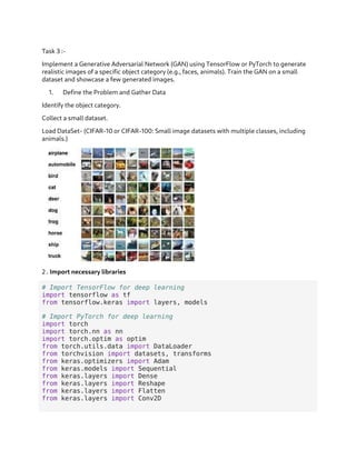
  • 6. # Setup the subplot formatting fig, ax = plt.subplots(ncols=10, figsize=(30,30)) # Loop four times and get images for idx in range(10): # Grab an image and label sample = dataiterator.next() # Plot the image using a specific subplot ax[idx].imshow(np.squeeze(sample['image'])) # Appending the image label as the plot title ax[idx].title.set_text(sample['label']) # Scale and return images only def scale_images(data): image = data['image'] return image / 255 # Reload the dataset ds = tfds.load('cifar10', split='train') # Running the dataset through the scale_images preprocessing step ds = ds.map(scale_images) # Cache the dataset for that batch ds = ds.cache() # Shuffle it up ds = ds.shuffle(50000) # Batch into 128 images per sample ds = ds.batch(128) # Reduces the likelihood of bottlenecking ds = ds.prefetch(64) ds.as_numpy_iterator().next().shape (128, 32, 32, 3) # Load a dataset using TensorFlow Datasets def load_dataset(dataset_name, split='train', batch_size=32): dataset, info = tfds.load(name=dataset_name, split=split, with_info=True) dataset = dataset.shuffle(1000).batch(batch_size).prefetch(tf.data.AUTOTUNE) return dataset, info np.squeeze(dataiterator.next()['image']).shape (32, 32, 3)
  • 7. # Example: Load the CIFAR-100 dataset dataset_name = 'cifar100' train_dataset, info = load_dataset('cifar100') # Visualize a few images from the dataset def visualize_dataset(dataset, num_samples=5): for data in dataset.take(1): images = data['image'][:num_samples].numpy() labels = data['label'][:num_samples].numpy() for i in range(num_samples): plt.subplot(1, num_samples, i + 1) plt.imshow(images[i]) plt.title(f"Label: {labels[i]}") plt.axis('off') plt.show() # Visualize the loaded CIFAR-100 dataset visualize_dataset(train_dataset) Downloading and preparing dataset 160.71 MiB (download: 160.71 MiB, generated: 132.03 MiB, total: 292.74 MiB) to /root/tensorflow_datasets/cifar100/3.0.2... {"model_id":"6cea445f9b904e3dbb604a96fa8a5dac","version_major":2,"vers ion_minor":0} {"model_id":"314b300cdbbe4a49955dbed15405c68f","version_major":2,"vers ion_minor":0} {"model_id":"6d8544d499414a8c861399b9286b1583","version_major":2,"vers ion_minor":0} {"model_id":"32349f6158b64c9fbc4e2d825fb91c93","version_major":2,"vers ion_minor":0} {"model_id":"65e9e60959124b9ab66d58c4edfafaad","version_major":2,"vers ion_minor":0} {"model_id":"42824834bf2040b5aa757600b77ff121","version_major":2,"vers ion_minor":0} {"model_id":"f59fe13314fa43d99549238922db3ff4","version_major":2,"vers ion_minor":0} {"model_id":"935ac3680f4c476885673c98b7b31448","version_major":2,"vers ion_minor":0} Dataset cifar100 downloaded and prepared to /root/tensorflow_datasets/cifar100/3.0.2. Subsequent calls will reuse this data.
  • 8. 4 . Build Generator and Discriminator Networks Define generator and discriminator architectures. Implement a Generative Adversarial Network (GAN) using TensorFlow Generative Adversarial Networks (GANs) Overview: Objective: The primary goal of a Generative Adversarial Network (GAN) is to generate new data samples that resemble a given training dataset. GANs consist of two neural networks, a generator, and a discriminator, which are trained together in a competitive manner. Components: Generator: The generator takes random noise as input and generates synthetic data samples. It starts with random noise and gradually refines its output to resemble real data. Discriminator: The discriminator is a binary classifier that distinguishes between real and generated data. It is trained to classify real data as real (label 1) and generated data as fake (label 0). Training Process: Generator Training:
  • 9. The generator aims to produce data that is indistinguishable from real data. It takes random noise as input and generates synthetic samples. The generator's objective is to fool the discriminator into classifying its output as real. Discriminator Training: The discriminator is trained on a mix of real and generated data. It learns to correctly classify real data as real and generated data as fake. The discriminator's objective is to correctly classify the source of the data. Build Neural Network 3.1 import modelling Components # Bring in the sequential api for the generator and discriminator from tensorflow.keras.models import Sequential # Bring in the layers for the neural network from tensorflow.keras.layers import Conv2D, Dense, Flatten, Reshape, LeakyReLU, Dropout, UpSampling2D # Generator model def build_generator(latent_dim, img_shape): model = models.Sequential() model.add(layers.Dense(256, input_dim=latent_dim)) model.add(layers.LeakyReLU(alpha=0.01)) model.add(layers.Reshape((8, 8, 4))) # Adjust the dimensions based on your requirements model.add(layers.Conv2DTranspose(128, kernel_size=4, strides=2, padding="same")) model.add(layers.LeakyReLU(alpha=0.01)) model.add(layers.Conv2DTranspose(64, kernel_size=4, strides=2, padding="same")) model.add(layers.LeakyReLU(alpha=0.01)) model.add(layers.Conv2DTranspose(1, kernel_size=4, strides=2, padding="same", activation="sigmoid")) return model # Discriminator model def build_discriminator(img_shape): model = models.Sequential() model.add(layers.Conv2D(64, kernel_size=4, strides=2, padding="same", input_shape=img_shape)) model.add(layers.LeakyReLU(alpha=0.01)) model.add(layers.Conv2D(128, kernel_size=4, strides=2, padding="same")) model.add(layers.LeakyReLU(alpha=0.01)) model.add(layers.Flatten()) model.add(layers.Dense(1, activation="sigmoid")) return model # Define the GAN model def build_gan(generator, discriminator): discriminator.trainable = False # Freeze discriminator weights
  • 10. during GAN training model = models.Sequential() model.add(generator) model.add(discriminator) return model # Set up the models latent_dim = 100 # Dimensionality of the random noise vector img_shape = (64, 64, 1) # Adjust based on your image size and channels generator = build_generator(latent_dim, img_shape) discriminator = build_discriminator(img_shape) # Compile discriminator (use binary crossentropy for a binary classification task) discriminator.compile(optimizer=tf.keras.optimizers.Adam(learning_rate =0.0002, beta_1=0.5), loss='binary_crossentropy', metrics=['accuracy']) # Compile the GAN model discriminator.trainable = False gan = build_gan(generator, discriminator) gan.compile(optimizer=tf.keras.optimizers.Adam(learning_rate=0.0002, beta_1=0.5), loss='binary_crossentropy') # Display model summaries generator.summary() discriminator.summary() gan.summary() Model: "sequential_4" _________________________________________________________________ Layer (type) Output Shape Param # ================================================================= dense_3 (Dense) (None, 256) 25856 leaky_re_lu_6 (LeakyReLU) (None, 256) 0 reshape_2 (Reshape) (None, 8, 8, 4) 0 conv2d_transpose_6 (Conv2D (None, 16, 16, 128) 8320 Transpose) leaky_re_lu_7 (LeakyReLU) (None, 16, 16, 128) 0 conv2d_transpose_7 (Conv2D (None, 32, 32, 64) 131136 Transpose)
  • 11. leaky_re_lu_8 (LeakyReLU) (None, 32, 32, 64) 0 conv2d_transpose_8 (Conv2D (None, 64, 64, 1) 1025 Transpose) ================================================================= Total params: 166337 (649.75 KB) Trainable params: 166337 (649.75 KB) Non-trainable params: 0 (0.00 Byte) _________________________________________________________________ Model: "sequential_5" _________________________________________________________________ Layer (type) Output Shape Param # ================================================================= conv2d_3 (Conv2D) (None, 32, 32, 64) 1088 leaky_re_lu_9 (LeakyReLU) (None, 32, 32, 64) 0 conv2d_4 (Conv2D) (None, 16, 16, 128) 131200 leaky_re_lu_10 (LeakyReLU) (None, 16, 16, 128) 0 flatten_1 (Flatten) (None, 32768) 0 dense_4 (Dense) (None, 1) 32769 ================================================================= Total params: 165057 (644.75 KB) Trainable params: 0 (0.00 Byte) Non-trainable params: 165057 (644.75 KB) _________________________________________________________________ Model: "sequential_6" _________________________________________________________________ Layer (type) Output Shape Param # ================================================================= sequential_4 (Sequential) (None, 64, 64, 1) 166337 sequential_5 (Sequential) (None, 1) 165057 ================================================================= Total params: 331394 (1.26 MB) Trainable params: 166337 (649.75 KB) Non-trainable params: 165057 (644.75 KB) _________________________________________________________________ img = generator.predict(np.random.randn(4,128,1)) 1/1 [==============================] - 0s 300ms/step
  • 12. 3.2 . Build Generator Networks import numpy as np import matplotlib.pyplot as plt from tensorflow.keras.models import Sequential from tensorflow.keras.layers import Dense, Reshape, BatchNormalization, LeakyReLU, Conv2DTranspose, Conv2D, Flatten def build_generator(latent_dim): model = Sequential() # Project and reshape the random input model.add(Dense(128 * 7 * 7, input_dim=latent_dim)) model.add(Reshape((7, 7, 128))) model.add(BatchNormalization()) model.add(LeakyReLU(0.2)) # Upsampling to generate a larger image model.add(Conv2DTranspose(128, kernel_size=4, strides=2, padding='same')) model.add(BatchNormalization()) model.add(LeakyReLU(0.2)) # Another upsampling layer model.add(Conv2DTranspose(128, kernel_size=4, strides=2, padding='same')) model.add(BatchNormalization()) model.add(LeakyReLU(0.2)) # Final convolutional layer to generate the output image model.add(Conv2D(1, kernel_size=7, activation='sigmoid', padding='same')) return model # Assuming you already have the generator model defined (e.g., using build_generator function) latent_dim = 128 unique_generator = build_generator(latent_dim) # Generate images using the unique generator generated_images = unique_generator.predict(np.random.randn(4, latent_dim)) # Setup the subplot formatting fig, ax = plt.subplots(ncols=4, figsize=(20, 20)) # Loop four times and get images for idx, img in enumerate(generated_images): # Plot the image using a specific subplot
  • 13. ax[idx].imshow(np.squeeze(img), cmap='gray') # Assuming grayscale images # Appending the image label as the plot title ax[idx].title.set_text(f"Generated Image {idx}") # Display the generated images plt.show() 1/1 [==============================] - 0s 202ms/step import numpy as np import matplotlib.pyplot as plt # Assuming you already have the generator model defined (e.g., using build_generator function) latent_dim = 128 unique_generator = build_generator(latent_dim) # Generate images using the unique generator generated_images = unique_generator.predict(np.random.randn(4, latent_dim, 1)) # Setup the subplot formatting fig, ax = plt.subplots(ncols=4, figsize=(20, 20)) # Loop four times and get images for idx, img in enumerate(generated_images): # Plot the image using a specific subplot ax[idx].imshow(np.squeeze(img), cmap='gray') # Assuming grayscale images # Appending the image label as the plot title ax[idx].title.set_text(f"Generated Image {idx}") # Display the generated images plt.show() 1/1 [==============================] - 0s 307ms/step WARNING:matplotlib.image:Clipping input data to the valid range for imshow with RGB data ([0..1] for floats or [0..255] for integers).
  • 14. WARNING:matplotlib.image:Clipping input data to the valid range for imshow with RGB data ([0..1] for floats or [0..255] for integers). WARNING:matplotlib.image:Clipping input data to the valid range for imshow with RGB data ([0..1] for floats or [0..255] for integers). WARNING:matplotlib.image:Clipping input data to the valid range for imshow with RGB data ([0..1] for floats or [0..255] for integers). 3.3 Build Discriminator Networks def build_discriminator(img_shape): model = Sequential() # Convolutional layers to process the input image model.add(Conv2D(64, kernel_size=3, strides=2, input_shape=img_shape, padding='same')) model.add(LeakyReLU(0.2)) model.add(Conv2D(128, kernel_size=3, strides=2, padding='same')) model.add(BatchNormalization()) model.add(LeakyReLU(0.2)) model.add(Conv2D(256, kernel_size=3, strides=2, padding='same')) model.add(BatchNormalization()) model.add(LeakyReLU(0.2)) # Flatten and dense layer for binary classification model.add(Flatten()) model.add(Dense(1, activation='sigmoid')) return model discriminator.summary() Model: "sequential_9" _________________________________________________________________ Layer (type) Output Shape Param # ================================================================= conv2d_15 (Conv2D) (None, 14, 14, 64) 640 leaky_re_lu_21 (LeakyReLU) (None, 14, 14, 64) 0
  • 15. conv2d_16 (Conv2D) (None, 7, 7, 128) 73856 leaky_re_lu_22 (LeakyReLU) (None, 7, 7, 128) 0 conv2d_17 (Conv2D) (None, 4, 4, 256) 295168 leaky_re_lu_23 (LeakyReLU) (None, 4, 4, 256) 0 flatten_2 (Flatten) (None, 4096) 0 dense_7 (Dense) (None, 1) 4097 ================================================================= Total params: 373761 (1.43 MB) Trainable params: 0 (0.00 Byte) Non-trainable params: 373761 (1.43 MB) _________________________________________________________________ img = img[0] img.shape (28, 3) # Assuming you already have the discriminator model defined (e.g., using build_discriminator function) discriminator = build_discriminator(img_shape=(28, 28, 3)) # Adjust img_shape based on your generated image size and channels # Generate color images using the unique generator generated_images = unique_generator.predict(np.random.randn(4, latent_dim, 1)) # Predict authenticity using the discriminator predictions = discriminator.predict(generated_images) # Display the discriminator predictions for idx, prediction in enumerate(predictions): print(f"Discriminator Prediction for Generated Image {idx}: {prediction}") 1/1 [==============================] - 0s 83ms/step 1/1 [==============================] - 0s 175ms/step Discriminator Prediction for Generated Image 0: [0.49947485] Discriminator Prediction for Generated Image 1: [0.49965706] Discriminator Prediction for Generated Image 2: [0.50006646] Discriminator Prediction for Generated Image 3: [0.4994955] 5 Loss Functions and Optimizers
  • 16. 1 Choose loss functions (e.g., Binary Crossentropy). 2 Set up optimizers for the generator and discriminator. from tensorflow.keras.layers import Flatten discriminator.add(Flatten()) discriminator.add(Dense(16384)) # Adjust the units based on your architecture from tensorflow.keras.models import Sequential from tensorflow.keras.layers import Dense, Flatten, LeakyReLU # Assuming you have a discriminator defined discriminator = Sequential() # Adjust input_shape based on the size of your images discriminator.add(Flatten(input_shape=(28, 28, 3))) discriminator.add(Dense(16384)) # Adjust the units based on your architecture discriminator.add(LeakyReLU(0.2)) # Add other layers as needed from tensorflow.keras.optimizers import Adam from tensorflow.keras.losses import BinaryCrossentropy from tensorflow.keras.models import Sequential # Assuming you have the generator and discriminator models defined generator = build_generator(latent_dim=128) discriminator = build_discriminator(img_shape=(64, 64, 3)) # Adjust img_shape based on your image size and channels # Define binary crossentropy loss function cross_entropy = BinaryCrossentropy(from_logits=True) # Set up optimizers for the generator and discriminator generator_optimizer = Adam(learning_rate=0.0002, beta_1=0.5) discriminator_optimizer = Adam(learning_rate=0.0002, beta_1=0.5) # Compile the discriminator discriminator.compile(optimizer=discriminator_optimizer, loss=cross_entropy, metrics=['accuracy']) # Assuming you have a discriminator defined discriminator = Sequential() # Adjust input_shape based on the size and channels of your images discriminator.add(Flatten(input_shape=(28, 28, 3))) discriminator.add(Dense(16384)) # Adjust the units based on your architecture discriminator.add(LeakyReLU(0.2)) # Add other layers as needed
  • 17. from tensorflow.keras.models import Sequential from tensorflow.keras.layers import Dense, Flatten, LeakyReLU # Assuming you have a discriminator defined discriminator = Sequential() # Adjust input_shape based on the size and channels of your images discriminator.add(Flatten(input_shape=(28, 28, 3))) discriminator.add(Dense(16384)) # Adjust the units based on your architecture discriminator.add(LeakyReLU(0.2)) # Add other layers as needed 6 . Train the GAN Loop through epochs. Loop through batches. Generate fake images with the generator. Train discriminator on real and fake images. Train generator to fool discriminator. Update weights based on losses. # Modify the generator to output images of shape (28, 28, 3) def build_generator(): model = Sequential() # ... (your existing generator architecture) model.add(Conv2D(3, kernel_size=3, activation='tanh', padding='same')) # Adjust the number of channels to 3 return model # Modify the discriminator to accept images of shape (64, 32, 32, 3) def build_discriminator(): model = Sequential() model.add(Conv2D(64, kernel_size=3, strides=2, input_shape=(64, 32, 32, 3), padding='same')) # ... (rest of your discriminator architecture) return model class CIFAR100GAN(Model): def __init__(self, generator, discriminator, *args, **kwargs): # Pass through args and kwargs to base class super().__init__(*args, **kwargs) # Create attributes for gen and disc self.generator = generator self.discriminator = discriminator
  • 18. def compile(self, g_opt, d_opt, g_loss, d_loss, *args, **kwargs): # Compile with base class super().compile(*args, **kwargs) # Create attributes for losses and optimizers self.g_opt = g_opt self.d_opt = d_opt self.g_loss = g_loss self.d_loss = d_loss def train_step(self, batch): # Get the data real_images = batch fake_images = self.generator(tf.random.normal((128, 128, 1)), training=False) # Train the discriminator with tf.GradientTape() as d_tape: # Pass the real and fake images to the discriminator model yhat_real = self.discriminator(real_images, training=True) yhat_fake = self.discriminator(fake_images, training=True) yhat_realfake = tf.concat([yhat_real, yhat_fake], axis=0) # Create labels for real and fakes images y_realfake = tf.concat([tf.zeros_like(yhat_real), tf.ones_like(yhat_fake)], axis=0) # Add some noise to the TRUE outputs noise_real = 0.15*tf.random.uniform(tf.shape(yhat_real)) noise_fake = -0.15*tf.random.uniform(tf.shape(yhat_fake)) y_realfake += tf.concat([noise_real, noise_fake], axis=0) # Calculate loss - BINARYCROSS total_d_loss = self.d_loss(y_realfake, yhat_realfake) # Apply backpropagation - nn learn dgrad = d_tape.gradient(total_d_loss, self.discriminator.trainable_variables) self.d_opt.apply_gradients(zip(dgrad, self.discriminator.trainable_variables)) # Train the generator with tf.GradientTape() as g_tape: # Generate some new images gen_images = self.generator(tf.random.normal((128,128,1)), training=True) # Create the predicted labels predicted_labels = self.discriminator(gen_images,
  • 19. training=False) # Calculate loss - trick to training to fake out the discriminator total_g_loss = self.g_loss(tf.zeros_like(predicted_labels), predicted_labels) # Apply backprop ggrad = g_tape.gradient(total_g_loss, self.generator.trainable_variables) self.g_opt.apply_gradients(zip(ggrad, self.generator.trainable_variables)) return {"d_loss":total_d_loss, "g_loss":total_g_loss} CIFAR100gan = CIFAR100GAN(generator, discriminator) # Compile the model CIFAR100gan.compile(g_opt, d_opt, g_loss, d_loss) Build Callback import os from tensorflow.keras.preprocessing.image import array_to_img from tensorflow.keras.callbacks import Callback class ModelMonitor(Callback): def __init__(self, num_img=3, latent_dim=128): self.num_img = num_img self.latent_dim = latent_dim def on_epoch_end(self, epoch, logs=None): random_latent_vectors = tf.random.uniform((self.num_img, self.latent_dim,1)) generated_images = self.model.generator(random_latent_vectors) generated_images *= 255 generated_images.numpy() for i in range(self.num_img): img = array_to_img(generated_images[i]) img.save(os.path.join('images', f'generated_img_{epoch}_{i}.png')) Train Model # Assuming your discriminator model looks like this model = Sequential() model.add(Conv2D(64, (3, 3), strides=(2, 2), padding="same", input_shape=(32, 32, 3)))
  • 20. import numpy as np import tensorflow as tf from tensorflow.keras import datasets, layers, models from tensorflow.keras.layers import Dense, Dropout, Activation, Flatten, Conv2D, MaxPooling2D (x_train, y_train) , (x_test, y_test) = datasets.cifar10.load_data() x_train = x_train.astype('float32') x_test = x_test.astype('float32') x_train /= 255.0 x_test /= 255.0 model = tf.keras.models.Sequential() model.add(tf.keras.layers.InputLayer(input_shape=(32,32,3))) model.add(tf.keras.layers.Conv2D(32, (3, 3), padding='same', activation='relu')) model.add(tf.keras.layers.MaxPooling2D(pool_size=(2, 2), strides=(2,2))) model.add(tf.keras.layers.Flatten()) model.add(tf.keras.layers.Dense(10, activation=tf.nn.softmax)) model.compile(loss='sparse_categorical_crossentropy', optimizer='adam', metrics=['accuracy']) model.summary() model.fit(x_train, y_train, batch_size=32, epochs=1) Model: "sequential_66" _________________________________________________________________ Layer (type) Output Shape Param # ================================================================= conv2d_82 (Conv2D) (None, 32, 32, 32) 896 max_pooling2d (MaxPooling2 (None, 16, 16, 32) 0 D) flatten_21 (Flatten) (None, 8192) 0 dense_47 (Dense) (None, 10) 81930 ================================================================= Total params: 82826 (323.54 KB) Trainable params: 82826 (323.54 KB) Non-trainable params: 0 (0.00 Byte) _________________________________________________________________ 1563/1563 [==============================] - 38s 24ms/step - loss: 1.4808 - accuracy: 0.4793 <keras.src.callbacks.History at 0x7d69ad81bb80>
  • 21. 7 Evaluate and Save Model Periodically evaluate generator's performance. Save generator and discriminator models. Review Performance import tensorflow as tf from tensorflow.keras import layers, models import matplotlib.pyplot as plt # Generator model definition def build_generator(noise_dim): model = models.Sequential() model.add(layers.Dense(7 * 7 * 256, use_bias=False, input_shape=(noise_dim,))) model.add(layers.BatchNormalization()) model.add(layers.LeakyReLU()) model.add(layers.Reshape((7, 7, 256))) assert model.output_shape == (None, 7, 7, 256) # Note: None is the batch size model.add(layers.Conv2DTranspose(128, (5, 5), strides=(1, 1), padding='same', use_bias=False)) assert model.output_shape == (None, 7, 7, 128) model.add(layers.BatchNormalization()) model.add(layers.LeakyReLU()) model.add(layers.Conv2DTranspose(64, (5, 5), strides=(2, 2), padding='same', use_bias=False)) assert model.output_shape == (None, 14, 14, 64) model.add(layers.BatchNormalization()) model.add(layers.LeakyReLU()) model.add(layers.Conv2DTranspose(1, (5, 5), strides=(2, 2), padding='same', use_bias=False, activation='tanh')) assert model.output_shape == (None, 28, 28, 1) return model # Instantiate the generator model noise_dim = 1000 generator = build_generator(noise_dim) # Generate images num_examples_to_generate = 16 seed = tf.random.normal([num_examples_to_generate, noise_dim]) predictions = generator(seed, training=False) # Display the generated images fig = plt.figure(figsize=(4, 4))
  • 22. for i in range(predictions.shape[0]): plt.subplot(4, 4, i+1) plt.imshow(predictions[i, :, :, 0], cmap='gray') plt.axis('off') plt.show() # Save the generator model generator.save('generator_model.h5') WARNING:tensorflow:Compiled the loaded model, but the compiled metrics have yet to be built. `model.compile_metrics` will be empty until you train or evaluate the model. # Assuming your discriminator model is defined and compiled def build_discriminator(img_shape): model = models.Sequential() model.add(layers.Conv2D(64, (5, 5), strides=(2, 2), padding='same', input_shape=img_shape)) model.add(layers.LeakyReLU(0.2)) model.add(layers.Dropout(0.3)) model.add(layers.Conv2D(128, (5, 5), strides=(2, 2), padding='same')) model.add(layers.LeakyReLU(0.2)) model.add(layers.Dropout(0.3)) model.add(layers.Flatten()) model.add(layers.Dense(1)) return model
  • 23. # Instantiate generator and discriminator noise_dim = 100 img_shape = (28, 28, 1) # Adjust according to your image shape generator = build_generator(noise_dim) discriminator = build_discriminator(img_shape) # Save generator and discriminator models generator.save('generator_model.h5') discriminator.save('discriminator_model.h5') WARNING:tensorflow:Compiled the loaded model, but the compiled metrics have yet to be built. `model.compile_metrics` will be empty until you train or evaluate the model. WARNING:tensorflow:Compiled the loaded model, but the compiled metrics have yet to be built. `model.compile_metrics` will be empty until you train or evaluate the model. 8 Generate and Showcase Images Use trained generator to generate new images. Display and showcase generated images. import tensorflow as tf import matplotlib.pyplot as plt # Replace 'path_to_your_generator_model' with the actual file path to your generator model generator = tf.keras.models.load_model('generator_model.h5') # Generate and showcase images generate_and_show_images(generator) WARNING:tensorflow:No training configuration found in the save file, so the model was *not* compiled. Compile it manually. 1/1 [==============================] - 0s 218ms/step
  • 24. Important Notes: Ensure proper model compilation and setup of loss functions and optimizers. Save and load models using model.save() and tf.keras.models.load_model(). Provide correct file paths when loading saved models. Adjust hyperparameters, architecture, and training settings based on your specific task. Feel free to customize the code snippets based on your dataset and requirements. Future scope The future scope of Generative Adversarial Networks (GANs) lies in addressing key challenges and expanding their applications. Research efforts are expected to focus on improving training
  • 25. stability, overcoming issues like mode collapse, and refining conditional GANs for more controlled image generation