1. Project 1, Shahin Esmail, 00828210
Computational PDEs: Final
1 Problem 1
1.1 Statement
Starting with the semi-Lagrangian advection code SemiLagrAdvect.m (written
for a rectangular domain and arbitrary ghost-point values), extend the program
to treat two-dimensional advection, governed by
∂q
∂t
+ ax
∂q
∂x
+ ay
∂q
∂y
= 0
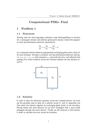
on a composite domain below by appropriately exchanging ghost point values af-
ter each timestep. Introduce a constant, but two-dimensional advection velocity,
i.e., (ax, ay) = (c1, c2) with constants c1,2 and verify the error- and reflection-free
passing of an initial condition across the interface between the two domains Ω1
and Ω2.
1.2 Solution
In order to solve the Advection equation across the L-shaped domain, we must
use the provided code to solve for a solution across Ω1 and Ω2 separately and
then patch the solution together by exchanging ghost points at the boundary.
Having solved over both domains we can then investigate how a wave would
propagate through the entire domain. Finally, we will construct a third domain
in order to calculate the error across the boundary.
1
2. 1.2 Solution Project 1, Shahin Esmail, 00828210
1.2.1 Solution over Ω1 and Ω2
Let us obtain a solution over Ω1, a 32 by 48 sided rectangle. In order to do this
we must set up our grid, matrix dimensions and boundary conditions. Similarly,
to obtain a solution over Ω2, a 64 by 32 sided rectangle, proceed in the same
way. Once created, we must patch the domains together by exchanging ghost
points at the boundary. In other words, we input the eastern ghost points of Ω1
into Ω2 and input the western ghost points of Ω2 into Ω1.
To implement this logic in Matlab, we must create a new driver that creates both
domains and within each time-step, patches a solution together.
First, construct both domains:
%% define the domain size
global xLen yLen xLen2 yLen2
global dx dy
global dt
ax = 0.1;
ay = -0.1;
%...domain size
xLen = 1;
yLen = 32/48;
xLen2 = 32/48;
yLen2 = 64/48;
Re = 500;
2
4. 1.2 Solution Project 1, Shahin Esmail, 00828210
uE1 = zeros(1,M1);
uW1 = zeros(1,M1);
vN1 = zeros(N1,1);
vS1 = zeros(N1,1);
vE1 = zeros(1,M1);
vW1 = zeros(1,M1);
%% define second domain
%define velocity
u2 =ax*ones(N2,M2); u2 = u2(:);
v2 =ay*ones(N2,M2); v2 = v2(:);
% boundary conditions
uN2 = zeros(N2,1);
uS2 = zeros(N2,1);
uE2 = zeros(1,M2);
uW2 = zeros(1,M2);
vN2 = zeros(N2,1);
vS2 = zeros(N2,1);
vE2 = zeros(1,M2);
vW2 = zeros(1,M2);
Now we must enter the advection loop. Within each time-step we must exchange
the boundary points to update the solution. This is done in the following way:
%% Mixing
for i=1:100
count = count+1;
uast1 = uast1(:);
vast1 = vast1(:);
uast2 = uast2(:);
vast2 = vast2(:);
% advection
uast1 = SemiLagrAdvect1(u1,v1,uast1,uS1,uN
1,uW1,uE1,N1,M1);
vast1 = SemiLagrAdvect1(u1,v1,vast1,vS1,vN
1,vW1,vE1,N1,M1);
uast2 = SemiLagrAdvect2(u2,v2,uast2,uS2,uN
2,uW2,uE2,N2,M2);
vast2 = SemiLagrAdvect2(u2,v2,vast2,vS2,vN
2,vW2,vE2,N2,M2);
4
5. 1.2 Solution Project 1, Shahin Esmail, 00828210
uast1 = reshape(uast1,N1,M1);
vast1 = reshape(vast1,N1,M1);
uast2 = reshape(uast2,N2,M2);
vast2 = reshape(vast2,N2,M2);
uW2(1,33:64) = transpose((uast1(N1,:)+uast2(1,33:64))/2);
vW2(1,33:64) = transpose((vast1(N1,:)+vast2(1,33:64))/2);
uE1 = (uast2(1,33:64)+uast1(N1,:))/2;
vE1 = (vast2(1,33:64)+vast1(N1,:))/2;
%plot the result
u = [[NaN*zeros(48,32), uast1];uast2];
v = [[NaN*zeros(48,32), vast1];vast2];
figure(3)
surf(xx,yy,sqrt(u.ˆ2+v.ˆ2));
axis([0 (1+32/48) 0 (64/48) -2 2]);
drawnow
end
Here uast1, vast1 represent the solution from Ω1 and uast2, vast2 represent the
solution from Ω2 which are updated in each time-step according to the boundary
by taking the average value between each solution.
1.2.2 SemiLagrangeAdvect.m
Notice in the code that there are now two versions of SemiLagrangeAdvect which
each correspond to Ω1 and Ω2 respectively. The difference between files is minor
however we must account for the corner point that lies on the top of the boundary.
5
6. 1.2 Solution Project 1, Shahin Esmail, 00828210
For Ω1 we include:
%...set the ghost values (four corners)
qq(1,1) = -qq(2,2);
qq(N+2,1) = -qq(N+1,2);
qq(N+2,M+2) = 2-qq(N+1,M+1);
qq(1,M+2) = -qq(2,M+1);
and similarly for Ω2:
%...set the ghost values (four corners)
qq(1,1) = -qq(2,2);
qq(N+2,1) = -qq(N+1,2);
qq(N+2,M+2) = -qq(N+1,M+1);
qq(1,M+2) = 2-qq(2,M+1);
1.2.3 Results:
Let us consider a flow with velocity (0.1, −0.1) through the L-shaped domain.
Using a surf plot we can visualise the result:
6
7. 1.2 Solution Project 1, Shahin Esmail, 00828210
Error:
Construct a third domain Ω3, a 32 by 80 sided rectangle and compute the dif-
ference between the solution of advection through it and that of the previous
domain. If our previous solution is patched correctly, we hope to find that the
error is negligible. Construct Ω3 and consider a flow with velocity (0.1,-0.1):
%% define the domain size
global xLen3 yLen3
%...domain size
xLen3 = 80/48;
yLen3 = 32/48;
% define third domain
N3 = 80;
M3 = 32;
%define the grid
x3 = linspace(0,xLen3,N3+1);
y3 = linspace(0,yLen3,M3+1);
xc3 = (x3(1:end-1)+x3(2:end))/2;
yc3 = (y3(1:end-1)+y3(2:end))/2;
7
8. 1.2 Solution Project 1, Shahin Esmail, 00828210
[yy3,xx3] = meshgrid(yc3,xc3);
%define the advection velocity
u3 = ax*ones(N3,M3); u3 = u3(:);
v3 = ay*ones(N3,M3); v3 = v3(:);
% boundary conditions
uN3 = ones(N3,1);uS3 = zeros(N3,1);
uE3 = zeros(1,M3);uW3 = zeros(1,M3);
vN3 = zeros(N3,1);vS3 = zeros(N3,1);
vE3 = zeros(1,M3);vW3 = zeros(1,M3);
Q3= zeros(N3,M3);
Q3(18:25,12:18) = 0;
Q3 = Q3(:);
uast3 = Q3;
vast3 = Q3;
count = 0;
for i=1:300
% advection
uast3 = SemiLagrAdvect(u3,v3,uast3,uS3,uN3,uW3,uE3,N3,M3);
vast3 = SemiLagrAdvect(u3,v3,vast3,vS3,vN3,vW3,vE3,N3,M3);
uast3 = reshape(uast3,N3,M3);
vast3 = reshape(vast3,N3,M3);
end
Calculate the residual values that resemble the error between the two solutions
which both propagate at a speed of (1, −1):
diffu = uast3 - u(1:80,33:64)
diffv = vast3 - v(1:80,33:64);
%%
residualu = norm(diffu)
residualv = norm(diffv)
Which yields the following error. Hence we can conclude that our solution from
patching together two separate domains is accurate.
residualu =
5.5831e-16
8
9. Project 1, Shahin Esmail, 00828210
2 Problem 2
2.1 Statement
Starting with the multigrid diusion code DiffusionSolve.m, generalize the program
to solve the two-dimensional diusion equation
∂q
∂t
= D(
∂2
q
∂x2
+
∂2
q
∂y2
)
on a composite domain by applying the multiplicative version of the alternating
Schwarz algorithm. Choose the overlap region indicated in the gure and pass the
solution along the respective interfaces as boundary conditions for the solution
on the individual domains Ω1 and Ω2. On the external boundary of the composite
domain, impose the Dirichlet boundary conditions. Verify your numerical solu-
tion by monitoring the residual on the interface. Select an appropriate diusion
coeffiecient D and advance your solution over a given time-interval T.
2.2 Solution
To solve this problem we must consider an overlap region between domains.
The idea of this solution is to extract solution values of one domain and input
them into the boundary of the other. In the way, we can patch the solution
correctly to explore how a wave would diffuse across this domain.
9
10. 2.2 Solution Project 1, Shahin Esmail, 00828210
2.2.1 Driver
As before, construct a second driver and define the first and second domain:
global xLen yLen xLen2 yLen2
global dx dy
global dt Re
%...domain size
xLen = 1;
yLen = 32/48;
xLen2 = 32/48;
yLen2 = 64/48;
N1 = 64;
M1 = 32;
N2 = 32;
M2 = 64;
x1 = linspace(0,xLen,48+1);
y1 = linspace(0,yLen,M1+1);
xc1 = (x1(1:end-1)+x1(2:end))/2;
yc1 = (y1(1:end-1)+y1(2:end))/2;
xxk1 = linspace(0,xLen,N1+1);
xxc1 = (xxk1(1:end-1)+xxk1(2:end))/2;
[yy1,xx1] = meshgrid(yc1,xxc1);
x2 = linspace(0,xLen2,N2+1);
y2 = linspace(0,yLen2,M2+1);
xc2 = (x2(1:end-1)+x2(2:end))/2;
yc2 = (y2(1:end-1)+y2(2:end))/2;
[yy2,xx2] = meshgrid(yc2,xc2);
[yy,xx] = meshgrid(yc2,[xc1 xc2+xLen]);
dx = xLen/48;
dy = dx;
dt = dx/1.5;
%...Reynolds number
Re = 500;
%...setup the hierarchy of R,A,P
[Rd1,Pd1,ilevmin1] = getRPd(N1,M1);
[Ad1, AAA1] = getAd(N1,M1,Rd1,Pd1);
10
12. 2.2 Solution Project 1, Shahin Esmail, 00828210
Ubc2(N2,:) = uE2*dt/Re/dx/dx;
Ubc2(:,1) = uS2*dt/Re/dy/dy;
Ubc2(:,M2) = uN2*dt/Re/dy/dy;
Vbc2 = zeros(N2,M2);
Vbc2(1,:) = vW2*dt/Re/dx/dx;
Vbc2(N2,:) = vE2*dt/Re/dx/dx;
Vbc2(:,1) = vS2*dt/Re/dy/dy;
Vbc2(:,M2) = vN2*dt/Re/dy/dy;
%initialise the solution
U1d = zeros(N1,M1);
V1d = zeros(N1,M1);
U2d = zeros(N2,M2);
V2d = zeros(N2,M2);
We now enter the time-loop where we patch together the solution. We must
modify the eastern boundary of Ω1 and the western boundary of Ω2. To do this,
we take the average value of the points that lie on either side of each boundary.
The time-step proceeds as follows:
for i = 1:400
diff1 = 1;
extractU1old = 0;
count = count+1;
countw = 0;
while diff1 > 10ˆ-6
countw = countw+1
%eastern boundary on omega 1
Ubc1(64,:) = (U2d(16,33:64)+U2d(17,33:64))*
dt/Re/dx/dx/2;
Vbc1(64,:) = (V2d(16,33:64)+V2d(17,33:64))*
dt/Re/dx/dx/2;
%southern boundary of omega 1
Ubc1(49:64,1) = (U2d(1:16,32)+U2d(1:16,33))*dt
/Re/dx/dx/2;
Vbc1(49:64,1) = (V2d(1:16,32)+V2d(1:16,33))*dt
/Re/dy/dy/2;
%west boundary of omega2
Ubc2(1,33:64) = (U1d(48,1:32)+U1d(49,1:32))*dt
/Re/dx/dx/2;
Ubc2(1,64) =(Ubc2(1,64)+Ubc1(49,32));
Vbc2(1,33:64) = (V1d(48,:)+V1d(49,:))*dt/Re/dy/dy/2;
Vbc2(1,64) = (Vbc2(1,64)+Vbc1(49,32));
12
14. 2.2 Solution Project 1, Shahin Esmail, 00828210
figure(3)
surf(xx,yy,sqrt(u.ˆ2+v.ˆ2));
drawnow
end
end
Notice we require convergence which is represented by the internal while loop.
We notice that we exit the while loop when the error between the old and the
new solution is greater than 10−6
.
2.2.2 Results
The following diagram shows how a patch diffuses through time:
14
15. 2.2 Solution Project 1, Shahin Esmail, 00828210
Which yields the last plot:
Finally, this yields the following residual plot:
15
16. Project 1, Shahin Esmail, 00828210
3 Problem 3
3.1 Statement
Starting with the multigrid Poisson solver PoissonSolve.m, generalize the program
to solve the two-dimensional Poisson equation
∂2
q
∂2x
+
∂2
q
∂2x
= f(x, y)
on a composite domain by applying the multiplicative version of the alternating
Schwarz algorithm. Choose the overlap region indicated in the gure and pass the
solution along the respective interfaces as boundary conditions for the solution
on the individual domains Ω1 and Ω2. On the external boundary of the com-
posite domain, impose homogeneous Neumann boundary conditions. Verify your
numerical solution by monitoring the residual on the interface.
3.1.1 Solution
Like in part 2 we must consider an overlap region and extract solutions to input
as boundary values. This time, using the logic from project 1, we must consider
the overlap region as a Dirichlet boundary condition and the external boundary
as a Neumann condition.
In order to solve the problem we must create two sets of the provided files to
account for Ω1 and Ω2.
16
17. 3.1 Statement Project 1, Shahin Esmail, 00828210
3.1.2 Changes to getAp
Recall from project 1 that a coefficient of -1 when defining the A matrix rep-
resents a Dirichlet condition and a -3 represents a Dirichlet condition. From
the diagram above, we require to change the Neumann boundary conditions on
the internal overlap region to Dirichlet. Hence for getAp, we must extract the
correct entries in both domains and change the coefficient such that the matrix
corresponds to the updated required boundary conditions. The extraction for
each boundary is shown as below:
Ω1 :
%...Laplace operator
AAx = spdiags(ones(N,1)*[1 -2 1]/dx/dx,-1:1,N,N);
AAx(1,1) = -1/dx/dx;
AAx(N,N) = -3/dx/dx;
AAy = spdiags(ones(M,1)*[1 -2 1]/dy/dy,-1:1,M,M);
AAy(1,1) = -1/dy/dy;
AAy(M,M) = -1/dy/dy;
AAx1 = kron(speye(M),AAx);
AAy2 = kron(AAy,speye(N));
for j = 49:64;
AAy2(j,j) = -3/dx/dx;
end
AAA = AAx1 + AAy2;
Ω2 :
%...Laplace operator
AAx = spdiags(ones(N,1)*[1 -2 1]/dx/dx,-1:1,N,N);
AAx(1,1) = -1/dx/dx;
AAx(N,N) = -1/dx/dx;
AAy = spdiags(ones(M,1)*[1 -2 1]/dy/dy,-1:1,M,M);
AAy(1,1) = -1/dy/dy;
AAy(M,M) = -1/dy/dy;
AAx1p1 = kron(speye(M),AAx);
AAx(1,1) = -3/dx/dx;
AAx1p2 = kron(speye(M),AAx);
AAy1p1 = kron(AAy,speye(N));
17
18. 3.1 Statement Project 1, Shahin Esmail, 00828210
AAx1 = [AAx1p1(1:1024,:);AAx1p2(1025:2048,:)];
AAy1p1(2048,2048) = -3/dx/dx;
AAx1(2048,2048) = -3/dx/dx;
AAA = AAx1 + AAy1p1;
3.1.3 Changes to getRP
Much like the above, we must modify our prolongation matrices so that we take
the new boundary into consideration. From project 1, a coefficient of 1
2
corre-
sponds to a Dirichlet condition and a coefficient of 2 corresponds to a Neumann.
Considering Ω1 and Ω2 separately we get:
Ω1
%...set up prolongation
NN = N/2;
MM = M/2;
for i=1:kl
PPx = sparse(2*NN,NN);
for j=1:NN-1
PPx(2*j:2*j+1,j:j+1) = [0.75 0.25; 0.25 0.75];
end
PPx(1,1) = 1;
PPx(2*NN,NN) = 1;
PPy = sparse(2*MM,MM);
for j=1:MM-1
PPy(2*j:2*j+1,j:j+1) = [0.75 0.25; 0.25 0.75];
end
PPy(1,1) = 1;
PPy(2*MM,MM) = 1;
Pp{i} = kron(PPy,PPx);
NN = NN/2;
MM = MM/2;
end
Ω2
%...set up prolongation
NN = N/2;
MM = M/2;
for i=1:kl
18
19. 3.1 Statement Project 1, Shahin Esmail, 00828210
PPx = sparse(2*NN,NN);
for j=1:NN-1
PPx(2*j:2*j+1,j:j+1) = [0.75 0.25; 0.25 0.75];
end
PPx(1,1) = 1;
PPx(2*NN,NN) = 1;
PPy = sparse(2*MM,MM);
for j=1:MM-1
PPy(2*j:2*j+1,j:j+1) = [0.75 0.25; 0.25 0.75];
end
PPy(1,1) = 1;
PPy(2*MM,MM) = 1;
Pp{i}=kron(PPy,PPx);
NN = NN/2;
MM = MM/2;
end
3.1.4 Driver
Construct the Driver for part 3 in the following way:
%%
global xLen yLen xLen2 yLen2
global dx dy
% global N1 M1 N2 M2
global Re
%...Reynolds number
Re = 500;
iteration = 10;
%...domain size
% xLen = 1;
% yLen = 32/64;
%
% xLen2 = 32/64;
% yLen2 = 1;
xLen = 1;
yLen = 32/64;
xLen2 = 32/64;
yLen2 = 1;
19
20. 3.1 Statement Project 1, Shahin Esmail, 00828210
N1 = 64;
M1 = 32;
N2 = 32;
M2 = 64;
% for the plotting I do not want the overlaps?
x1 = linspace(0,48/64,48+1);
y1 = linspace(0,yLen,M1+1);
xc1 = (x1(1:end-1)+x1(2:end))/2;
yc1 = (y1(1:end-1)+y1(2:end))/2;
xxk1 = linspace(0,xLen,N1+1);
xxc1 = (xxk1(1:end-1)+xxk1(2:end))/2;
[yy1,xx1] = meshgrid(yc1,xxc1);
x2 = linspace(0,xLen2,N2+1);
y2 = linspace(0,yLen2,M2+1);
xc2 = (x2(1:end-1)+x2(2:end))/2;
yc2 = (y2(1:end-1)+y2(2:end))/2;
xc = [xc1, xc2+48/64];
[yy2,xx2] = meshgrid(yc2,xc2);
[yy,xx] = meshgrid(yc2,xc);
dx = xLen/N1;
dy = yLen/M1;
%%
% set up the first domain
% define the prolongation and restriction matrices
[Rp1,Pp1] = getRPp1(N1,M1);
Ap1 = getAp1(N1,M1,Rp1,Pp1);
p0x1 = zeros(N1,M1);
% I choose as function f = xˆ2+yˆ2,
the poisson Dfˆ2/Dˆ2x + Dfˆ2/Dˆ2y
% rhs = -sin(2*pi*xx).*sin(2*pi*yy);
rhs = ones(80,64);
% rhs = yy./((1+xx).ˆ2+yy.ˆ2);
rhs1 = rhs(1:N1,1:M1);
% set up the second domain
[Rp2,Pp2] = getRPp2(N2,M2);
Ap2 = getAp2(N2,M2,Rp2,Pp2);
p0x2 = zeros(N2,M2);
%...right-hand side and initial guess
20
23. 3.1 Statement Project 1, Shahin Esmail, 00828210
3.1.5 Results:
Let us consider how the solution converges over 10 iterations. We hope that the
solution smooths out over the entire domain.
The first three iterations are as follows:
After 10 iterations we find:
23
24. 3.1 Statement Project 1, Shahin Esmail, 00828210
Residual
Finally, monitoring the residual on the interface we obtain the following plot:
Notice that this plot is similar to the plot for question 2 in magnitude as some
error in the code has been carried forward.
24
25. Project 1, Shahin Esmail, 00828210
4 Problem 4
4.1 Statement
Combine your three codes above to solve incompressible flow in an L-shaped
driven cavity. By operator splitting, we solve the incompressible Navier-Stokes
equation
∂u
∂t
+ u u = − p +
1
Re
2
u
u = 0
with u = (u, v) as the two-dimensional velocity field, p as the pressure, and Re
denoting the Reynolds number, in four steps.
To solve this part we must amend the file cavityflow.m such that the L-shaped
domain is taken into consideration.
4.1.1 Part (1) & (2)
Solve the advection part over one time-step using your code from Problem 1.
Subsequently, use the result of the advection step as an initial condition for one
time-step with the diffusion code from Problem 2.
To tackle this problem we must obatin a solution from the advection code and
pass that solution through to the diffusion code. This can be done with the
following code:
global xLen yLen xLen2 yLen2
global dx dy dt
% global N1 M1 N2 M2
global Re
%...Reynolds number
Re = 500;
% added driver Q1 while it still has a glitch
%...domain size
xLen = 1;
yLen = 32/64;
xLen2 = 32/64;
yLen2 = 1;
N1 = 64;
25
30. 4.1 Statement Project 1, Shahin Esmail, 00828210
extractU1new = U1d(49:64,:);
diff1 = norm(extractU1new - extractU1old);
extractU1old = U1d(49:64,:);
diff1;
end
u1d = U1d;
u2d = U2d;
v1d = V1d;
v2d = V2d;
udraw = [[NaN*zeros(48,32), u1d(1:48,:)];u2d];
vdraw = [[NaN*zeros(48,32), v1d(1:48,:)];v2d];
figure(10)
contourf(xx,yy,sqrt(udraw.ˆ2+vdraw.ˆ2))
drawnow
pause
For one time step this code advects the solution to obatin a uast,vast and then
places that value into diffusion.
4.1.2 Part (3)
Use the output (u,v) from the diffusion step to solve the Poisson equation (using
your code from Problem 3) for the pressure p such that
f(x, y) =
∂u
∂x
+
∂v
∂y
Again, pass the solution obtained from above to solve the Poisson equation
in the following way. Compute the divergence and proceed using the logic from
lectures:
% ...computing divergence
uS1new = [uS1;Ubc1(49:64,1)];
vS1new = [vS1;Vbc1(49:64,1)];
30
32. 4.1 Statement Project 1, Shahin Esmail, 00828210
PBd1(64,32) = PBd1(64,32)+PBd2(16,64);
p0x1 = p0x1new;
p0x2 = p0x2new;
extractponew = p0x1(49:64,:);
residual = norm(extractponew - extractpoold);
extractpoold = p0x1(49:64,:);
end
4.1.3 Part (4)
Correct the (u,v)-field from step 3 according to
u ← u +
∂p
∂x
v ← v +
∂p
∂y
and commence with the next time-step.
Choose the dimensions indicated in figure 1(b) and a Reynolds number of Re =
500 and solve for the velocity field (u, v). Advance the solution in time suffi-
ciently long for a steady state to form. Visualize your results and experiment
with the Reynolds number. Identify and describe all vortices in your domain.
Finally correct the velocities appropriately and exit the end the first time-step
using the following code:
%% ...correcting velocities
vS1new = [vS1d;PBd1(49:64,1)];
vE1new = PBd1(64,:);
[px1,py1] = Diff(p0x1new(:),N1,M1,'N',vS1new,vN1,vW1,vE1new);
U1final = U1d(:) - px1(:);
V1final = V1d(:) - py1(:);
vW2new = [vW2(1:32),PBd2(1,33:64)];
[px2,py2] = Diff(p0x2new(:),N2,M2,'N',vS2,vN2,vW2new,vE2);
U2final = U2d(:) - px2(:);
V2final = V2d(:) - py2(:);
32
33. 4.1 Statement Project 1, Shahin Esmail, 00828210
U1final = reshape(U1final,N1,M1);
V1final = reshape(V1final,N1,M1);
U2final = reshape(U2final,N2,M2);
V2final = reshape(V2final,N2,M2);
%%
u1 = U1final(1:48,:);
v1 = V1final(1:48,:);
u2 = U2final;
v2 = V2final;
if (mod(i,2)==0)
udraw = [[NaN*zeros(48,32), U1final(1:48,:)];U2final];
vdraw = [[NaN*zeros(48,32), V1final(1:48,:)];V2final];
fprintf('time step %i n',i)
figure(2)
quiver(xx(1:k:end,1:k:end),yy(1:k:end
,1:k:end),udraw(1:k:end,1:k:end),vdra
w(1:k:end,1:k:end),12/k)
axis image
drawnow
figure(3)
surf(xx,yy,sqrt(udraw.ˆ2+vdraw.ˆ2))
drawnow
end
end
Modification to Diff.m
Update the code in the following way:
function [qx,qy] = Diff(q,N,M,typ,qS,qN,qW,qE)
global dx dy
qq = reshape(q,N,M);
qG = zeros(N+2,M+2);
qG(2:N+1,2:M+1) = qq;
33
34. 4.1 Statement Project 1, Shahin Esmail, 00828210
if (typ=='D')
qG(1,2:M+1) = 2*qW-qG(2,2:M+1);
qG(N+2,2:M+1) = 2*qE-qG(N+1,2:M+1);
qG(2:N+1,1) = 2*qS-qG(2:N+1,2);
qG(2:N+1,M+2) = 2*qN-qG(2:N+1,M+1);
elseif (typ=='N')
qG(1,2:M+1) = qG(2,2:M+1);
qG(N+2,2:M+1) = qG(N+1,2:M+1);
qG(2:N+1,1) = qG(2:N+1,2);
qG(2:N+1,M+2) = qG(2:N+1,M+1);
end
qx = (qG(3:N+2,2:M+1)-qG(1:N,2:M+1))/(2*dx);
qy = (qG(2:N+1,3:M+2)-qG(2:N+1,1:M))/(2*dy);
Combining this all yields the following fluid flow for Re = 500:
34
35. 4.1 Statement Project 1, Shahin Esmail, 00828210
After a significent number of iterations, (400), the solution stabilizes to the
following flow:
We notice there are two main vortices, one in Ω1 and one in Ω2.
On increasing Re = 10000 we notice that the vortices form much more slowly.
This can be seen on comparing the 100th iteration with the previous case:
35