![7.2
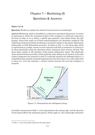
angle) is zero, the resulting process is referred to as orthogonal cutting. If not, it is said
to be oblique cutting.
Question: How do we apply these concepts to turning?
Answer: In turning, three basic motions are needed to cut the workpiece:
i) Spindle speed (N) [rev/min] or [rpm]: It is the rotational speed of the
spindle/chuck that provides the primary motion in turning. Since the workpiece
is directly attached on to the spindle, this speed gives rise to the cutting velocity
(v) in [m/s]:
𝑣 = 𝑅Ω = 𝑅
2𝜋𝑁
60 (7.1)
where R [m] is the radial position of the cutting tool; [rad/s] denotes the angular
speed of the spindle.
ii) Feed (or feed-rate) (f) [mm/rev]: Feed, which provides the secondary motion
in turning, is defined as the axial displacement of the tool for each revolution of
the workpiece. Since [rev] is not considered to be a physical unit, f is generally
specified in [mm]. Thus, revolution is implied in that case. Note that the feed
implicitly corresponds to the axial speed of the tool (u) in [m/s]:
𝑢 =
𝑓𝑁
60 ⋅ 1000 (7.2)
iii) Depth-of-cut (d) [mm]: This quantity specifies the diametric depth of material
to be removed on the workpiece. Hence, users can control the shape of part
through a series of adjustments on this parameter. Please note that since we
shall only deal with the outer/inner diameter turning in this course, this
parameter is treated as a constant for all practical purposes.
As a consequence of these motions, the cutting tool moves on a helical path with respect
to the workpiece. Now, let us explain the chip production in turning. Fig. 7.2d illustrates
a typical outer diameter (OD) turning operation. Fig. 7.2a shows the view from the cross-
slide side. Here, the tool is continuously fed onto the rotating workpiece by f mm per each
revolution. Different cross-sections of the tool (into paper plane) engage into cut. This is
the plane in which the major cutting action is performed. Note that the cutting edge of
the tool resembles the wedge illustrated in Fig. 7.1. Similarly, 7.2c demonstrates the
upper view of the conducted operation. As highlighted in this figure, the tool has two
cutting edges:
a) Major (or side) cutting edge,
b) Minor (or end) cutting edge.
The major cutting edge cuts the workpiece sideways along the axial direction (z) (refer
to Fig. 7.2c). Similarly, the minor cutting edge cuts the workpiece radially as shown in
Fig. 7.2b. In other words, the tool separates the material in tangential direction. In fact,
the geometry around the intersection point of these edges (a.k.a. tool nose) determines
the surface quality of the turned part. Contrary to the representation in Fig. 7.2c, a typical
tool is not infinitely sharp and has a round nose in practice. Anyway, we shall come back
to that issue later.](data:image/gif;base64,R0lGODlhAQABAIAAAAAAAP///yH5BAEAAAAALAAAAAABAAEAAAIBRAA7)
Recommended
More Related Content
Similar to Chapter 7 - Q A (v2.2) .pdf
Similar to Chapter 7 - Q A (v2.2) .pdf (20)
Recently uploaded
Recently uploaded (20)
Chapter 7 - Q A (v2.2) .pdf
- 1. 7.1 Chapter 7 – Machining (I) Questions & Answers Slides 7.3-7.6 Question: Would you explain the material removal process in machining? Answer: Machining, which is classified as a subtractive manufacturing process, is a series of operations in which the unwanted portion of the workpiece is selectively removed in the form of chips so as to obtain a specific part geometry and surface finish. For this purpose, sharp tools made out of hard metals/substances are oftentimes employed. The underlying mechanism behind machining is somewhat similar to the plastic deformation taking place in bulk deformation processes. As shown in Fig. 7.1, the sharp edge, which is represented as a wedge, stresses out the material such that it commences to yield (or to be shorn plastically) along the directions where maximum shear stresses develop. The shear plane resides on the frontline of this plastic deformation region. The plastically shorn material behaves just like a deck of playing cards sliding on one another as the rake surface compresses the material to yield. It eventually produces the deformed chip (i.e. a strip/ribbon) that extends outwards beginning from the shear plane. It is self-evident that to shear (i.e “cut”) the material, a relative motion between the tool and workpiece is required. Deformed Chip Tool Shear Angle: Φ Normal Rake Angle: γn Undeformed Chip Thickness: a c Figure 7.1: Nomenclature for orthogonal cutting. As briefly summarized in Slide 7.4, the angle between the cutting edge1 and the direction of tool motion affects the machining process. If this angle (i.e. the cutting edge inclination 1 In Fig. 7.1, the cutting edge extends into the paper plane.
- 2. 7.2 angle) is zero, the resulting process is referred to as orthogonal cutting. If not, it is said to be oblique cutting. Question: How do we apply these concepts to turning? Answer: In turning, three basic motions are needed to cut the workpiece: i) Spindle speed (N) [rev/min] or [rpm]: It is the rotational speed of the spindle/chuck that provides the primary motion in turning. Since the workpiece is directly attached on to the spindle, this speed gives rise to the cutting velocity (v) in [m/s]: 𝑣 = 𝑅Ω = 𝑅 2𝜋𝑁 60 (7.1) where R [m] is the radial position of the cutting tool; [rad/s] denotes the angular speed of the spindle. ii) Feed (or feed-rate) (f) [mm/rev]: Feed, which provides the secondary motion in turning, is defined as the axial displacement of the tool for each revolution of the workpiece. Since [rev] is not considered to be a physical unit, f is generally specified in [mm]. Thus, revolution is implied in that case. Note that the feed implicitly corresponds to the axial speed of the tool (u) in [m/s]: 𝑢 = 𝑓𝑁 60 ⋅ 1000 (7.2) iii) Depth-of-cut (d) [mm]: This quantity specifies the diametric depth of material to be removed on the workpiece. Hence, users can control the shape of part through a series of adjustments on this parameter. Please note that since we shall only deal with the outer/inner diameter turning in this course, this parameter is treated as a constant for all practical purposes. As a consequence of these motions, the cutting tool moves on a helical path with respect to the workpiece. Now, let us explain the chip production in turning. Fig. 7.2d illustrates a typical outer diameter (OD) turning operation. Fig. 7.2a shows the view from the cross- slide side. Here, the tool is continuously fed onto the rotating workpiece by f mm per each revolution. Different cross-sections of the tool (into paper plane) engage into cut. This is the plane in which the major cutting action is performed. Note that the cutting edge of the tool resembles the wedge illustrated in Fig. 7.1. Similarly, 7.2c demonstrates the upper view of the conducted operation. As highlighted in this figure, the tool has two cutting edges: a) Major (or side) cutting edge, b) Minor (or end) cutting edge. The major cutting edge cuts the workpiece sideways along the axial direction (z) (refer to Fig. 7.2c). Similarly, the minor cutting edge cuts the workpiece radially as shown in Fig. 7.2b. In other words, the tool separates the material in tangential direction. In fact, the geometry around the intersection point of these edges (a.k.a. tool nose) determines the surface quality of the turned part. Contrary to the representation in Fig. 7.2c, a typical tool is not infinitely sharp and has a round nose in practice. Anyway, we shall come back to that issue later.
- 3. 7.3 f d Tool N A-A Cross-section Chip Flow u d Tool Tangential Direction Workpiece N B-B Cross-section Ro Ri (a) Front-view (Cross-slide side) (b) Side-view (Tailstock side) d A A B B N Tool Workpiece Major edge Minor edge r z Chip Flow Chip d Tool D0 Di v f N (c) Top-view (Top of the lathe) (d) 3D configuration (adapted from [3]) Figure 7.2: Chip formation in OD (or cylindrical) turning.
- 4. 7.4 Slides 7.11-7.13 Question: Why are we so interested in machining forces? Answer: Measurement and estimation of machining forces is a big deal. They play a key role in many different aspects of manufacturing including: i) Prediction of tool wear and breakage; ii) Evaluation of machinability; iii) Chatter detection; iv) Machining process monitoring / optimization; v) Adaptive control of CNC machine tools; vi) Machine tool design; vii) Cutting tool design and more. Question: How do we get to measure these forces in practice? Would you also show where these forces actually develop on an actual turning process? Answer: In turning, the force components (Fc, Ft, and Frad), which are shown in Fig. 7.3, can be conveniently measured by employing a load cell. In this (offline) measurement scheme, the load cell housing the cutting tool is attached on to the cross-slide of the lathe2. While machining, the output of the load cell (either voltage or current) is amplified, sampled, and recorded. The saved data are then transformed to get these force components in [N]. f d Tool Fc Ft d Tool Workpiece N Frad Fc (a) Front-view (Cross-slide side) (b) Side-view (Tailstock side) Figure 7.3: Machining force components acting on the tool. The measurement of the other force pairs is very convoluted. Therefore, once Fc, Ft (and Frad) are obtained, the other projections are estimated using mathematical models such as the ones presented in Slide 7.12. In fact, these (projected) force pairs enable us to investigate the effects of stresses on other critical elements of machining (e.g. tool, chip, workpiece). Fig. 7.4 illustrates the free body diagrams associated with the orthogonal 2 Your second lab exercise will be on this topic.
- 5. 7.5 cutting process. As can be seen from the diagram on the right, the rake surface force components (Fn and Ff) initiating the machining process naturally develop on the tool. That is, Ff is created by the friction process as the chip rubs against the rake surface while the normal force (Fn) is caused by the reaction of the chip resisting to the plastic deformation. Consequently, the resultant force (Fr) on the rake is presumed to be directly transferred to the chip which in return compresses the material into yield on the shear surface (refer to the diagram in the middle). Evidently, Fr conveyed onto the chip- workpiece interface can be resolved into the force pairs Fs and Fns. Here, Fs generates the shearing stresses for instigating the plastic deformation while Fns produces the pressure building on the shear plane. The main cutting force (Fc) and the feed force (Ft) components are simply the horizontal- and vertical projections of the reaction force to the shear plane elements (see the diagram in the left). Notice that since the actual geometry of the turning tool (and/or the shear plane) is pretty complicated, it is quite difficult to show the above- mentioned force pairs on a diagram like Fig. 7.3. Deformed Chip Tool Φ γn Fc Ff Fn Fr Fr Ft Fs Fns Fr Fc Fr Ft Workpiece Fs Fns Ff Fn Fr Fr ac v a0 vc β β Figure 7.4: Free body diagrams of orthogonal cutting process (adapted from [7]). Slides 7.18-7.21 Question: Would you explain Lee-Shaffer’s theory? Answer: To understand the theory, consider the shear zone model shown in Fig. 7.5a (see also Slide 7.21). As can be seen, the resultant force (Fr) acting on the rake surface (i.e. the chip-tool interface) compresses the material in the triangular zone such that the material yields along the shear plane and that the maximum shear stresses are induced along the slip lines parallel to this shear plane. Since the model presumes that the direction of the maximum principal stress (1) coincides with the action line of the resultant force, the orientation of the slip lines with respect to the rake surface can be obtained.
- 6. 7.6 To illustrate the determination of the shear plane angle () using this theory, let us consider the simplified geometry in Fig. 7.5b. Here, the angle B can be directly found as 90– from the geometry around point B. Since the slip lines, which are parallel to the shear plane, must make an angle of 45 with the action line of the resultant force; the angle C is immediately read as 45. β Φ 45o σ1 γn Fr θ = 45o 90o -γn 45o +β σ1 σ2 σ2 90o -γn 90o -β 90o -β β Φ 45o 45o A B C 45o +β (a) Shear zone model (b) Simplified geometry Figure 7.5: Lee-Shaffer’s shear model. Now, two of the inner angles for the triangle ABC are known. The remaining angle becomes 𝐴 ̂ = 180° − 𝐵 ̂ − 𝐶 ̂ = 180° − (90° − 𝛽) − 45° ∴ 𝐴 ̂ = 45° + 𝛽 As the last step, the angles around point A should add up to 180. Evidently, Φ = 45° − 𝛽 + 𝛾𝑛 Question: It is claimed that neither the Lee-Shaffer’s nor the Ernst-Merchant’s theories about the shear-plane angle is in good agreement with the experiments? What is the reason for this discrepancy? Answer: As can be seen from Fig. 7.6, the predictions of both theories are not always in accordance with the experimental results. One obvious reason for this mismatch is that both theories rely on pure geometry to estimate the shear plane angle. In other words, they do not include any parameters representing the (thermo)-mechanical behavior of the workpiece material (or the tool itself)3. Furthermore, both theories adopt a thin-shear zone model where the material is plastically shorn along a thin plane. Unfortunately, this assumption is not very realistic. The experiments show that the material is shorn inside a relatively thick zone and that the chip formation using a simple wedge-like tool is surprisingly a very complicated process. Notice that the methods that we have effectively used to analyze the plastic deformation in bulk-forming processes are not too fruitful in machining owing to the fact that the flow-direction of the material is not well-constrained here. For short, a single shear plane is simply a theoretical 3 Some researchers (including Eugene Merchant himself) did attempt to incorporate the mechanical behavior of the stressed material to the shear-plane theory. However, they obtained limited success.
- 7. 7.7 abstraction to help us understand some basic features of the machining. Consequently, more advanced theories have yet to be developed to bridge this apparent gap. Figure 7.6: Shear angles obtained through experiments on various materials [6]. Slide 7.22 Question: Would you explain the geometry of the undeformed chip? Answer: Fig. 7.7a illustrates the area of undeformed chip. This is the area of which the major cutting edge directly faces to (see also Fig. 7.2a). Here, the angle (), which is called side cutting edge angle (or the lead angle), controls the cutting process and the corresponding chip geometry. If it is zero, the process is referred to as orthogonal cutting. Otherwise, it turns into oblique cutting as explained in Slide 7.4. We can derive some important relationships by employing the geometry in Fig. 7.7b. For instance, the undeformed chip thickness (ac) is 𝑎𝑐 = 𝑓𝑐𝑜𝑠(𝜅) (7.3) Similarly, the width of the chip (aw) becomes 𝑎𝑤 = 𝑑 𝑐𝑜𝑠(𝜅) (7.4) It is critical to note that the area of the undeformed chip (Ac) (i.e. the area of the parallelogram) can be obtained as 𝐴𝑐 = 𝑓𝑑 (7.5) Hence, the side cutting edge angle () does not have an influence on this area.
- 8. 7.8 d κ Workpiece Tool f f ac κ d aw κ (a) Area of the undeformed chip (b) Enlarged cross-section Figure 7.7: Simplified geometry of undeformed chip. Question: How do we define MRR? Answer: MRR is defined as the volume of material being removed per unit time. For turning process, the (swept) volume can be easily computed: 𝑀𝑅𝑅 = 𝑤 = 𝐴𝑐𝑣 (7.6) where v = R [see Eqn. (7.1)] refers to the cutting speed. Substituting Eqn. (7.5) into (7.6) gives 𝑀𝑅𝑅 = 𝑓𝑑𝑣 (7.7) Note that the cutting speed refers to the circumferential velocity of the workpiece with respect to the cutting tool and varies as a function of R. For OD turning, we compute v = R0 under the assumption4 that R0 >> d (refer to Fig. 7.2b). If d is relatively large, the cutting velocity should be calculated as 𝑣 = 𝑅0 + 𝑅𝑖 2 Ω = (𝑅0 − 𝑑 2 ) Ω (7.8) Slide 7.27 Question: Why is the specific cutting energy (E) decreasing as the undeformed chip thickness (ac) and/or the cutting speed (v) increases? Isn’t it counter-intuitive? Answer: No, it is not. Let us start our discussion with the effect of cutting speed. Machining energy is actually a very complicated physical quantity that happens to be affected by many diverse factors such as tool/workpiece material, tool geometry, lubrication conditions, interface temperature, etc. Therefore, the reason why the cutting speed directly influences the energy is a very complex one. We shall greatly simplify the explanation given here. 4 Unless instructed otherwise in the exams, this is the default method to compute the cutting speed for OD turning.
- 9. 7.9 Assuming that the energy is decomposed into two components: i) energy needed to plastically shear the material (in primary shear zone); ii) energy to overcome friction at the rake- and flank surfaces. As the cutting velocity increases, the strain-rate (𝜀̇𝑝𝑙) is expected to increase. In fact, in metal cutting literature, Johnson-Cook stress-strain relationship is commonly used: 𝜎𝑓(𝜀𝑝𝑙, 𝜀̇𝑝𝑙, 𝑇) = [𝜎𝑓0 + 𝐾′ (𝜀𝑝𝑙) 𝑛′ ] ⏟ strain dependence [1 + 𝐶 ln ( 𝜀̇𝑝𝑙 𝜀̇𝑟𝑒𝑓 )] ⏟ strain-rate dependence [1 − ( 𝑇 − 𝑇𝑟𝑒𝑓 𝑇𝑚𝑒𝑙𝑡 − 𝑇𝑟𝑒𝑓 ) 𝑚′ ] ⏟ temperature dependence (7.9) Here, 𝜎𝑓0, 𝐾′ ≠ 𝐾, 𝐶, 𝑛′ ≠ 𝑛, 𝑚′ ≠ 𝑚 are the material coefficients to be determined experimentally; 𝑇𝑚𝑒𝑙𝑡[°𝐶] refers the melting temperature of the material; 𝑇𝑟𝑒𝑓 ≤ 𝑇 ≤ 𝑇𝑚𝑒𝑙𝑡 is the working temperature. In practice, 𝑇𝑟𝑒𝑓 = 𝑇𝑟𝑜𝑜𝑚; 𝜀̇𝑟𝑒𝑓 = 1. The corresponding shear stress can be expressed as 𝜏𝑠 ≅ 𝜎𝑓 2 ∝ (𝜀𝑝𝑙) 𝑛′ 𝜀̇𝑝𝑙 (7.10) Hence, as 𝜀̇𝑝𝑙 increase, the shear stress in yield (𝜏𝑠) along with its associated work tends to grow as well. On the other hand, high interface temperatures (600C–1000C) are usually attained as a consequence of high velocity5. They would reduce the overall proportionality coefficient 𝐶𝐾′ [1 − ( 𝑇−𝑇𝑟𝑒𝑓 𝑇𝑚𝑒𝑙𝑡−𝑇𝑟𝑒𝑓 ) 𝑚′ ] (i.e. the flow stress accordingly) in Eqn. (7.9). All in all, the energy may tend to drop with increasing cutting speeds6 (see also Slide 3.25). Likewise, the friction energy, which apparently dominates its counterpart, exhibits a tendency to decrease as cutting speed rises. To explain that, we shall presume that the work done against friction is correlated to the effective friction coefficient at the workpiece-tool interface. From your physics classes, you might recall Stribeck curve which defines the (kinetic) friction coefficient as a function of the contact speed. At low speeds, the friction coefficient (at the boundary lubrication region) is pretty high while it rapidly drops down at moderate velocities where mixed lubrication kicks in. As the velocity really builds up, a fluid cushion develops between the contacting media and hydrodynamic lubrication becomes effective. Same analogy could be employed in this case except that the cutting fluids (lubricants) do not exactly behave as described by Stribeck curve. In extreme cases, solid-to-solid contact between the tool and workpiece becomes eminent. In such situations, high interface temperature may lower the frictional shear stress as suggested above. Consequently, the resulting specific cutting energy could go down as illustrated in this slide. With respect to the effect of undeformed chip thickness (ac) on the specific cutting energy, E can be expressed in terms of ac as explained in Slide 7.25: 𝐸 = 𝐹𝑐cos(𝜅) 𝑎𝑐𝑑 ∝ 𝑎𝑐 −1 (7.11) Hence, E is inversely proportional to ac in theory. 5 Fig. 8-10 of Ref. [1] shows the temperature effects as a function of cutting speed. 6 Not everybody agrees with that statement. Ref. [2] suggests that the two effects (i.e. high strain rates and high temperatures) on the shear plane cancel each other.
- 10. 7.10 Slide 7.28 Question: So far, we have only concentrated on the turning process. Is it possible to extend these concepts to milling? How can we compute the average force and power in milling? Answer: We can extend all of these concepts to milling. Fig. 7.8 illustrates a typical end- milling process that utilizes a flat-end mill with four cutting edges (or flutes). Taking a close look at the cross-section of the helical tool in the figure reveals that each of these edges (at a particular height/elevation) resembles a single-point turning tool. The only difference here is that the tool is both rotating and translating simultaneously with respect to the workpiece. Consequently, the cross-section of the chip changes dynamically while the developed forces vary periodically as different cutting edges engage / disengage into cut. That poses some challenge in deriving dynamic process models. The (simplified) model presented here is essentially based on specific cutting energy and yields the average machining force in end-milling operations. The main/tangential force component (Fc) can be expressed as 𝐹𝑐 = 𝑘𝑐 ⏟ 𝐸 (𝑧𝑒𝑏ℎ𝑚) ⏟ 𝐴𝑐 (7.12) Here, kc is the specific cutting energy [N/mm2]; b is the chip width [mm]; hm is the average chip thickness along its width [mm]; 𝑧𝑒 ∈ ℝ refers to the fraction of flutes engaged into cut: 𝑏 = 𝑎𝑝 cos(𝜆) (7.13a) ℎ𝑚 = 𝑓𝑧(𝑎𝑒2 − 𝑎𝑒1) 𝑅𝜑 (7.13b) 𝑧𝑒 = 𝑧𝑛 𝜑 2𝜋 (7.13c) where R is the radius of the cutter [mm]; is the helix angle; (0 ae1 2R) and (ae1 ae2 2R) are the dimensions defining the radial depth of cut [mm]; ap is the (axial) depth of cut [mm]; 𝑧𝑛 ∈ ℕ is the number of edges (flutes) on the cutting tool while fz denotes the feed-per-tooth [mm/tooth]: 𝑓𝑛 ≜ 𝑓𝑧𝑧𝑛 (7.14) In Eqn. (7.14), fn is referred to as the feed-per-revolution [mm/rev]. The immersion or sweep angle () in Eqns. (7.13b) and (7.13c) can be expressed as = cos−1 (1 − 𝑎𝑒2 𝑅 ) − cos−1 (1 − 𝑎𝑒1 𝑅 ) (7.15) However, it is self-evident that does not play any role in average force computation owing to the fact that the product ℎ𝑚𝑧𝑒 in Eqn. (7.12) becomes independent from .
- 11. 7.11 ap Workpiece Tool Cutting Edge λ ae1 ae2 u R x y N θ 1 2 3 4 1 2 3 ϕ γ Figure 7.8: Nomenclature for a generic end-milling process. The specific cutting energy respective to a particular cut in Eqn. (7.12) is commonly modified as follows: 𝑘𝑐 = 𝑘𝑐11(ℎ𝑚)−𝑚𝑐 (1 − 0.01𝛾𝑜 ) ⏟ correction factor (7.16) where o is the (radial) rake angle in degrees (see Fig. 7.8); kc11 [N/mm2] is the specific cutting energy for 1 mm of (undeformed) chip thickness and 1 mm of chip width (when utilizing a tool with o = 0); 0 < mc < 1 indicates the pressure conversion exponent7. Notice that the specific cutting energy (kc11) is highly correlated with the yield strength of the material. Since increasing the hardness of a material via certain processes (i.e. heat treatment, plastic deformation, aging, alloying, etc.) is known to extend its elastic limit (i.e. pushing the yield strength above that of the annealed state), kc11 is often times shown as a function of the material type as well as overall hardness in metal cutting literature. The tool catalogs of various manufacturers tabulate these constants (kc11 and mc) for key engineering metals. The machining power in [W] can be simply calculated as 𝑃spindle = 𝐹𝑐𝑣 (7.17) where the circumferential speed of the tool (v) [m/s] is 𝑣 = 2𝜋𝑅𝑁 6 ⋅ 104 (7.18) Here, N refers to the rotational speed of the cutting tool [rpm]. Combining Eqns. (7.12)– (7.14), (7.17), and (7.18) yields 𝑃spindle = 𝑘𝑐 (𝑧𝑛𝑓 𝑧𝑁) ⏟ 𝑢 (𝑎𝑒2 − 𝑎𝑒1)𝑎𝑝 6 ⋅ 104 cos(𝜆) (7.19) In fact, the same result would have been obtained by using the basic definition of MRR: 7 The symbols are modified here to maintain compatibility with the metal cutting literature (i.e. especially, the tool catalogs). For instance, according to our course-note convention, kc11 E (for ac = 1 mm); mc .
- 12. 7.12 MRR = 𝑤 = (𝑎𝑒2 − 𝑎𝑒1) 𝑎𝑝 cos(𝜆) ⏟ 𝑏 𝑢 (7.20) It is critical to note that the term (𝑎𝑒2 − 𝑎𝑒1) 𝑎𝑝 cos(𝜆) in Eqn. (7.20) essentially denotes the area swept by the tool. By definition, the feed-rate (u) [mm/min] is 𝑢 ≜ 𝑓𝑛𝑁 = 𝑧𝑛𝑓𝑧𝑁 (7.21) Since 𝑃spindle = 𝑘𝑐 ⏟ 𝐸 𝑤, (7.22) plugging Eqns. (7.20) and (7.21) into (7.22) yields 𝑃spindle = 𝑘𝑐(𝑧𝑓𝑧𝑁) (𝑎𝑒2 − 𝑎𝑒1)𝑎𝑝 6 ⋅ 104 ⏟ conversion factor cos(𝜆) (7.23) This expression is identical to Eqn. (7.19). Notice that the average values of the force components Fx, Fy, and Fz are interrelated to Fc via a large number of different parameters. Based on experimental studies, Ref. [4] recommends the followings: 𝐹𝑥 = 𝐹𝑢 = { (1 … 1.2)𝐹𝑐, for up-milling (0.8 … 0.9)𝐹𝑐, for down-milling (7.24a) 𝐹𝑦 = 𝐹radial = { (0.2 … 0.3)𝐹𝑐, for up-milling (0.75 … 0.8)𝐹𝑐, for down-milling (7.24b) 𝐹𝑧 = 𝐹axial = 𝐹𝑐 tan(𝜆) (7.24c) However, equations like (7.24) are rarely used in practice. Fc is presumed to apply directly to the direction of interest as the worst-case scenario. For more information, please refer to Ref. [5] that introduces advanced methods to compute the dynamic machining forces. Slide 7.29 Question: What is the purpose of this table? Answer: The table in this slide was adapted from Ref. [1]. We have specifically included this table to give our students an insight about the magnitudes of specific cutting energy for different materials. As can be seen, E ranges between 0.2 [GPa] (Mg, zinc alloys) and 4.0 [GPa] (tool steels). Note that it is a good engineering practice to cross-check constantly the magnitudes as well as the units of the physical quantities in one’s calculations.
- 13. 7.13 Slide 7.30 Question: Would you give an example on the orthogonal cutting geometry and cutting/ machining forces? Answer: Consider the problem (Problem 1) in this slide. The given data are as follows: ac = 0.25 [mm] a0 = 0.75 [mm] d = 2.5 [mm] Fc = 900 [N] Ft = 450 [N] n = 10 a) Mean angle of friction on the rake (): (Slide 7.12) tan(𝛽 − 𝛾𝑛) = 𝐹𝑡 𝐹𝑐 = 450 900 = 0.5 𝛽 − 𝛾𝑛 = tan−1(0.5) = 26.565° 𝛽 = 26.565° + 10° = 36.565° b) Cutting ratio (rc): (Slide 7.13) 𝑟𝑐 = 𝑎𝑐 𝑎0 = 0.25 0.75 = 1 3 c) Shear angle (): (Slide 7.13) tan(Φ) = 𝑟𝑐 cos(𝛾𝑛) 1 − 𝑟𝑐 sin(𝛾𝑛) = 1 3 cos(10°) 1 − 1 3 sin(10°) = 0.345 Φ = tan−1(0.345) = 19.034° d) Shear plane forces (Fs, Fns): (Slide 7.12) 𝐹𝑠 = 𝐹𝑐 cos(Φ) − 𝐹𝑡 sin(Φ) = 900 cos(19.034°) − 450 sin(19.034°) Fs = 704.46 [N] 𝐹𝑛𝑠 = 𝐹𝑐 sin(Φ) + 𝐹𝑡 cos(Φ) = 900 sin(19.034°) + 450 cos(19.034°) Fns = 718.5 [N] e) Rake surface forces (Ff, Fn): (Slide 7.12) 𝐹𝑓 = 𝐹𝑐 sin(γn) + 𝐹𝑡 cos(γn) = 900 sin(10°) + 450 cos(10°) Ff = 599.45 [N] 𝐹𝑛 = 𝐹𝑐 cos(γn) − 𝐹𝑡 sin(γn) = 900 cos(10°) − 450 sin(10°) Fn = 808.19 [N] f) Friction coefficient (): (Slide 7.12) μ = tan(𝛽) = tan(36.565°) = 0.742
- 14. 7.14 Slide 7.31 Question: Would you give an example on the power requirement in machining? Answer: Consider the problem (Problem 2) in this slide. The given data are as follows: Pidle = 325 [W] Pcut = 2580 [W] N = 124 [rpm] v = 24.5 [m/min] f = 0.2 [mm/rev] d = 3.8 [mm] = 0 (orthogonal cutting!) = 0.4 a) Specific cutting energy (E): (Slide 7.25) E = 𝑃spindle 𝑤 = 𝑃cut − 𝑃idle ⏞ Net power available for turning 𝑣𝑓𝑑 ⏟ MRR = 2580 − 325 ⏞ [𝑊: 𝐽/𝑠] 24.5 ∙ 103 60 ⏟ [𝑚𝑚/𝑠] 0.2 ⏟ [𝑚𝑚] 3.8 ⏟ [𝑚𝑚] = 2255 310.333 𝐸 = 7.266 [J/mm3 : GPa] b) Torque at the spindle (Tspindle): For this calculation, we need the angular speed of the spindle: 𝛺 = 2𝜋𝑁 60 = 2𝜋 124 60 = 13 [rad/s] ∴ 𝑇spindle = 𝑃spindle 𝛺 = 2255 13 ⇒ 𝑇spindle = 173.659 [Nm] c) Cutting force (Fc): (Slide 7.25) 𝐹𝑐 = 𝑃spindle 𝑣 = 2255 24.5 60 ⏟ [𝑚/𝑠] ⇒ 𝐹𝑐 = 5522 [N] d) Specific cutting energy (E) for ac = 1 [mm]: (Slide 7.26) The specific cutting energy in part (a) is valid for an (undeformed) chip thickness of 𝑎𝑐 = 𝑓𝑐𝑜𝑠(𝜅) = 0.2 cos(0°) = 0.2 [mm]. We are asked to find E that corresponds to ac = 1 [mm]. Thus, 𝐸1 𝐸2 = ( 𝑎𝑐1 𝑎𝑐2 ) −𝛼 ⇒ 𝐸1 = 7.266 ( 1 0.2 ) −0.4 𝐸 = 𝐸1 = 3.817 [J/mm3 ]
- 15. 7.15 Slide 7.32 Question: Is the presented theory (on machining power) only applicable to turning process? Answer: The presented theory can be easily extended to other machining processes as well. For instance, the problem (Problem 3) in this slide is about drilling as illustrated in the figure. Let us first write down the given data: E = 77 [W/(cm3/min)] v = 24.5 [m/min] f = 0.2 [mm/rev] = 0.85 2R = 25 [mm] φ25 Twist Drill u N a) Motor power (Pmotor): (Slide 7.24) The key in solving this problem is to calculate the MRR for drilling. It can be conveniently defined as the product of the hole’s area (A) and the axial speed of the drill (u). The MRR (or w) essentially yields the volume swept by the twist drill per unit time. That is, 𝑤 = 𝐴𝑢 = 𝜋𝑅2 ⏟ 𝐴 (𝑓𝑁) ⏟ 𝑢 Unfortunately, the spindle speed (N) is not directly given in the problem. On the other hand, the cutting speed (v), which is the circumferential speed of the drill by definition, is specified. Hence, 𝑣 = 𝑅Ω = 𝑅 (2𝜋𝑁) ⏟ Ω ⇒ 𝑁 = 𝑣 2𝜋𝑅 = 24500 ⏞ [𝑚𝑚/𝑚𝑖𝑛] 𝜋 25 ⏟ [𝑚𝑚] 𝑁 = 312 [rpm] = 5.2 [rev/s] Using the first equation, we get 𝑤 = 𝜋(12.5)2(0.2 ⋅ 5.2) = 510 [mm3 /s] Spindle power is calculated as 𝑃spindle = 𝐸 𝑤 = 77 ⋅ 60 1000 ⏟ [J/mm3] 510 ⏟ [ mm3 s ] = 2356 [W] Consequently, the motor power becomes 𝑃motor = 𝑃spindle 𝜂 = 2356 0.85 = 2772 [W] b) Spindle torque (Tspindle): 𝑇spindle = 𝑃spindle 𝛺 = 2356 2𝜋 5.2 ⏟ [rad/s] ⇒ 𝑇spindle = 72.103 [Nm]
- 16. 7.16 Slide 7.33 Question: How about the example in the last slide? Answer: This problem (Problem 4) is newly added and is supposed to cover every topic in this chapter. Again, let us jot down the data of the problem: f0 = 600 [MPa] Fr = 800 [N] a0 = 0.8 [mm] f = 0.4 [mm/rev] d = 2 [mm] = 12 e = 8 n = 6 a) Friction coefficient on the rake surface (): (Slide 7.12) The friction coefficient requires the ratio of the cutting force components Ft and Fc (see Slide 7.12). Unfortunately, they are not directly specified in the problem. Based on the given data, our best bet is to find the (shear plane) force components (Fs, Fns) and work our way back to (Fc, Ft). Let us first obtain the shear angle: 𝑟𝑐 = 𝑎𝑐 𝑎0 = 𝑓𝑐𝑜𝑠(𝜅) 𝑎0 = 0.4 cos(12°) 0.8 = 0.4891 tan(Φ) = 𝑟𝑐 cos(𝛾𝑛) 1 − 𝑟𝑐 sin(𝛾𝑛) = 0.4891 cos(6°) 1 − 0.4891 sin(6°) = 0.5126 Φ = tan−1(0.5126) = 27.141° From Slide 7.16, the shear plane force can be expressed as 𝐹𝑠 = 𝜏𝑠 [ 𝐴𝑐 sin(Φ) ] ⏟ 𝐴𝑠 = 𝜏𝑠𝐴𝑐 sin(𝛷) ≅ 𝜎𝑓0 2 (𝑓𝑑) sin(𝛷) = 300 (0.4 ⋅ 2) sin(27.141) = 526.1299 [N] 𝐹𝑛𝑠 = √𝐹𝑟 2 − 𝐹𝑠 2 = √8002 − 526.12992 = 602.6502 [N] Employing the equations in Slide 7.12, we can write Fc and Ft in terms of Fs and Fns: 𝐹𝑐 = 𝐹𝑠 cos(Φ) + 𝐹𝑛𝑠 sin(Φ) = 526.1299 cos(27.141°) + 602.6502 sin(27.141°) Fc = 743.1140 [N] 𝐹𝑡 = −𝐹𝑠 sin(Φ) + 𝐹𝑛𝑠 cos(Φ) = −526.1299 sin(27.141°) + 602.6502 cos(27.141°) Ft = 296.2794 [N] Consequently, tan(𝛽 − 𝛾𝑛) = 𝐹𝑡 𝐹𝑐 = 296.2794 743.1140 = 0.3987 𝛽 − 𝛾𝑛 = tan−1(0.3987) = 21.7372° 𝛽 = 21.7372° + 6° = 27.7372° μ = tan(𝛽) = tan(27.7372°) = 0.5258
- 17. 7.17 Note that an alternative solution for this part is to employ either Ernst-Merchant’s or Lee-Shaffer’s theory to find directly after computing . Let us try them all: Ernst-Merchant: (Slide 7.17) 𝛽 = 90° − 2Φ + 𝛾𝑛 = 90° − 2 ⋅ 27.141° + 6° = 41.718° μ = tan(𝛽) = tan(41.718°) = 0.8915 Lee-Shaffer: (Slide 7.21) 𝛽 = 45° − Φ + 𝛾𝑛 = 45° − 27.141° + 6° = 23.859° μ = tan(𝛽) = tan(23.859°) = 0.4423 As can be seen, Lee-Shaffer’s model yields a closer result (to = 0.5258). b) Surface roughness (Rmax): (Slide 8.9) This portion is related to the next chapter. Anyway, the surface roughness is given in Slide 8.9 as 𝑅max = 𝑓 tan(𝜅) + cot(𝜅𝑒) = 0.4 tan(12°) + cot(8°) = 55 [μm] References [1] Schey, J. A., Introduction to Manufacturing Processes, 2nd Edition, McGraw Hill, NY, 1987. [2] Shaw, M. C., Metal Cutting Principles, 2nd Edition, Oxford University Press, Oxford, UK, 2005. [3] Girsang, I. P., Dhupia, J. S., “Machine Tools for Machining,” Handbook of Manufacturing Engineering and Technology, pp. 811-865, Springer-Verlag, London, 2015. [4] Akkurt, M., Machine Tools: Machining Methods and Technology (in Turkish), Birsen Publishing Co., Istanbul, 2000. [5] Altıntaş, Y., Manufacturing Automation, 2nd Edition, Cambridge University Press, Cambridge, UK, 2012. [6] Boothroyd, G., Knight, W. A., Fundamentals of Machining and Machine Tools, 2nd Edition, Marcel Dekker Inc., NY, 1989. [7] DeGarmo E. P., Black, J. T., Kohser, R.A., Materials and Processes in Manufacturing, 13th Edition, Wiley, NY, 2019.