
Recommended
More Related Content
What's hot
What's hot (19)
Similar to Round2: Maths Challenge organised by ‘rep2rep’ research group at Sussex&Cambridge universities
Similar to Round2: Maths Challenge organised by ‘rep2rep’ research group at Sussex&Cambridge universities (20)
Recently uploaded
Recently uploaded (20)
Round2: Maths Challenge organised by ‘rep2rep’ research group at Sussex&Cambridge universities
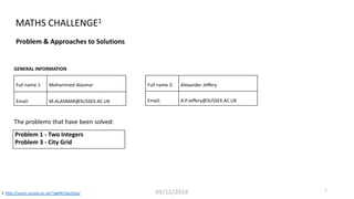
- 1. Full name 1: Mohammed Alasmar Email: M.ALASMAR@SUSSEX.AC.UK GENERAL INFORMATION Problem & Approaches to Solutions MATHS CHALLENGE1 http://users.sussex.ac.uk/~gg44/rep2rep/1 The problems that have been solved: Problem 1 - Two Integers Problem 3 - City Grid 1 09/12/2018 Full name 2: Alexander Jeffery Email: A.P.Jeffery@SUSSEX.AC.UK
- 2. 2 Problem 1 - Two Integers Two different integers between 1 and 10 are chosen at random. What is the probability that they are consecutive? Problem 3 - City Grid You and your friend live in a grid-like city. Every edge of the grid is a road. The distance from your place to your friend's place is n roads north and m roads east. You and your friend decide to visit each other but both of you leave at the same time and walk at the same speed. If both of you take 'optimal paths' (minimising the length of the paths), what's the probability that you will meet on your way?
- 3. Q1 3
- 4. 4 Index Number 1 Number 2 1 1 2 2 1 3 3 1 4 4 1 5 5 1 6 6 1 7 7 1 8 8 1 9 9 1 10 10 2 1 11 2 3 12 2 4 13 2 5 14 2 6 15 2 7 16 2 8 17 2 9 18 2 10 19 3 1 20 3 2 21 3 4 22 3 5 23 3 6 24 3 7 25 3 8 26 3 9 27 3 10 28 4 1 29 4 2 30 4 3 31 4 5 32 4 6 33 4 7 34 4 8 35 4 9 36 4 10 37 5 1 38 5 2 39 5 3 40 5 4 41 5 6 42 5 7 43 5 8 44 5 9 45 5 10 46 6 1 47 6 2 48 6 3 49 6 4 50 6 5 51 6 7 52 6 8 53 6 9 54 6 10 55 7 1 56 7 2 57 7 3 58 7 4 59 7 5 60 7 6 61 7 8 62 7 9 63 7 10 64 8 1 65 8 2 66 8 3 67 8 4 68 8 5 69 8 6 70 8 7 71 8 9 72 8 10 73 9 1 74 9 2 75 9 3 76 9 4 77 9 5 78 9 6 79 9 7 80 9 8 81 9 10 82 10 1 83 10 2 84 10 3 85 10 4 86 10 5 87 10 6 88 10 7 89 10 8 90 10 9 Case 1: Permutations without replacement i.e., the two numbers are different and order is considered, for example (1,2) and (2,1) should be taken in the outcome. We define the consecutive numbers as the numbers which follow each other in order, without gaps, from smallest to largest. Picking two different number between [1,10] gives 90 possible outcomes, where 9 of them represent the cases of getting consecutive numbers, as shown in Fig.1 (the yellow cells). Hence, the probability that the two numbers are consecutive can be found as follows: ! = 9 90 = #. % Fig.1
- 5. 5 1 2 3 4 5 6 7 8 9 10 1 2 3 4 5 6 7 8 9 10 1 2 3 4 5 6 7 8 9 10 1 2 3 4 5 6 7 8 9 10 Case 1: We define the consecutive numbers as the numbers which follow each other in order, without gaps, from smallest to largest. Fig.2(a) shows are the possible outcomes from picking two different number between [1,10]. These are represented by the black squares in the figure, which are 90 squares. The cases of consecutive numbers are represented by the yellow squares in Fig.2(b), which are 9 squares. Hence, the probability that the two numbers are consecutive can be found as follows: All outcomes (the black squares = 90) The cases of consecutive numbers (the yellow squares = 9) ! = number of yellow squares number of black squares = 9 90 = #. % Fig.2 Fig.2(a) Fig.2(b) Number 1 Number 1 Number2 Number2
- 6. 6 2 3 4 5 1 6 7 8 9 10 1 3 4 5 2 6 7 8 9 10 1/9 1/10 1/10 1 2 4 5 3 6 7 8 9 10 1 2 3 5 4 6 7 8 9 10 1/10 1/10 1 2 3 4 5 6 7 8 9 10 1 5 3 4 6 5 7 8 9 10 1/10 1/10 1 2 3 4 7 5 6 8 9 10 1 2 3 4 8 5 6 7 9 10 1/10 1/10 1 2 3 4 9 5 6 7 8 10 1 2 3 4 10 5 6 7 8 9 1/10 1/10 1/9 1/9 1/9 1/9 1/9 1/9 1/9 1/9 Case 1: The tree diagram is used in this solution (see below). The first stage in this tree (picking the first number at random) contains ten outcomes: [1:10], so the probability of each one of these outcomes is 1/10. In the second stage, 9 possible numbers can be selected at random. Only one of these 9 numbers is a consecutive number to the number that was selected at the first stage except for number 10 which does not have any consecutive number. Thus, the probability that the two numbers are consecutive can be found as follows: ! = #× 1 10 × % # = 1 10 = &. %
- 7. 7 The Permutation is defined as a selection of numbers in which the order of the numbers matters, and there is no replacement. This is the case of this question i.e., we solve it with order and without replacement. Hence, we can use the permutation formula to find the total number of possible outcomes, as follows: !(#, %) = # % = #! # − % ! 10 2 = 10! 10 − 2 ! = 90 Now, the number of choices with consecutive numbers = # − 1 = 10 − 1 = 9 This is because each number has a consecutive but not the last number (this is based on our definition of consecutive numbers, i.e., the consecutive numbers are the numbers which follow each other in order, without gaps, from smallest to largest) Therefore, the probability of choosing consecutive numbers is Case 1: ! = # − 1 #! # − % ! = 10 − 1 10! 10 − 2 ! = 9 90 = 0.1
- 8. 8 If we want to pick 2 different numbers from the set of numbers [1:10], then there are 10 options to pick from for the first number and 9 options for the second number, as shown in Fig.3. Thus, the total number of selections = number of available values for number 1 x number of available values for number 2 = 10 × 9 = 90 Now, for the first picked number there is only one consecutive number expect for the largest number, which does not have any consecutive number (see Fig.4). This means that there are 9 possibilities of getting consecutive numbers. Therefore, the probability of choosing consecutive numbers is & = 9 90 = '. ) 10 9 8 7 6 5 4 3 2 1 123456789 Case 1: Fig.3 the number of available numbers for picking 10 available Pick number 1 Pick number 2 9 available Fig.4 each number has a consecutive but not 10 No consecutive
- 9. 9 clc,close all x = 1:10; y = 1:10; counterAll = 0; counterCons = 0; for i=1:10 for j = 1:10 if y(j)==x(i)+1 plot(x(i),y(j),'rs','LineWidth', 15) counterCons = counterCons+1; end hold on if x(i)~=y(j) plot(x(i),y(j),'bd','LineWidth', 4) counterAll = counterAll+1; end end end grid on,xlabel('number 1'), ylabel('number 2') set(gca,'fontsize',15) legend('consecutive','all outcomes') prob = counterCons/counterAll prob = 0.1000 Running the code gives the probability value and Fig.5. By using the following Matlab code. Fig.5
- 10. 10 The second number is bigger than the first. If the first number is k (which happens with probability 1/n), then the probability the second number is 1/(n-1). Case 1 ! = # $%& '(& 1 * × 1 * − 1 ! = # $%& &-(& 1 10 × 1 9 = 9× 1 10 × 1 9 = 1 10 = 0.1
- 11. 11 Case 2: Solving the problem using combination, i.e., there is no replacement and order is not important, for example, we just take one of these groups (1,2) and (2,1). We define the consecutive numbers as the numbers which follow each other in order, without gaps, from smallest to largest. Picking two different number between [1,10] gives 90 possible outcomes, where 9 of them represent the cases of getting consecutive numbers, as shown in Fig.6 (the yellow cells). Hence, the probability that the two numbers are consecutive can be found as follows: ! = 9 45 = #. % Fig.6 Index Number 1 Number 2 1 1 2 2 1 3 3 1 4 4 1 5 5 1 6 6 1 7 7 1 8 8 1 9 9 1 10 10 2 3 11 2 4 12 2 5 13 2 6 14 2 7 15 2 8 16 2 9 17 2 10 18 3 4 19 3 5 20 3 6 21 3 7 22 3 8 23 3 9 24 3 10 25 4 5 26 4 6 27 4 7 28 4 8 29 4 9 30 4 10 31 5 6 32 5 7 33 5 8 34 5 9 35 5 10 36 6 7 37 6 8 38 6 9 39 6 10 40 7 8 41 7 9 42 7 10 43 8 9 44 8 10 45 9 10
- 12. 12 1 2 3 4 5 6 7 8 9 10 1 2 3 4 5 6 7 8 9 10 Case 2: We define the consecutive numbers as the numbers which follow each other in order, without gaps, from smallest to largest. Fig.7(a) shows are the possible outcomes from picking two different number between [1,10]. These are represented by the black squares in the figure, which are 45 squares. The cases of consecutive numbers are represented by the yellow squares in Fig.7(b), which are 9 squares. Hence, the probability that the two numbers are consecutive can be found as follows: All outcomes (the black squares = 45) The cases of consecutive numbers (the yellow squares = 9) ! = number of yellow squares number of black squares = 9 45 = #. % Fig.7 Fig.7(a) Fig.7(b) Number 1 Number 1 Number2 Number2 1 2 3 4 5 6 7 8 9 10 1 2 3 4 5 6 7 8 9 10
- 13. 13 2 3 4 5 1 6 7 8 9 10 3 4 5 2 6 7 8 9 10 4 5 3 6 7 8 9 10 5 4 6 7 8 9 10 5 6 7 8 9 10 6 7 8 9 10 7 8 9 10 8 9 10 9 10 Case 2: The tree diagram is used in this solution. The first stage in this tree (picking the first number at random) contains ten outcomes: [1:10], so the probability of each of these outcomes is 1/10. In the second stage, 9 possible numbers can be selected at random. Only one of these 9 numbers is a consecutive number to the number that was selected at the first stage except for number 10 which does not have any consecutive number. Now, the probability that the two numbers are consecutive can be found as follows: ! = number of consecutives total number of possible outcome = 3 45 = 6. 8
- 14. 14 The Combination is defined as a selection of numbers in which the order of the numbers does not matter, and there is no replacement. This is the case of this question i.e., without order and without replacement. Hence, we can use the Combination formula to find the total number of possible outcomes, as follows: ! ", $ = " $ = "! " − $ ! $! 10 2 = 10! 10 − 2 ! 2! = 45 Now, the number of choices with consecutive numbers = " − 1 = 10 − 1 = 9 This is because each number has a consecutive but not the last number (this is based on our definition of consecutive numbers, i.e., the consecutive numbers are the numbers which follow each other in order, without gaps, from smallest to largest) Therefore, the probability of choosing consecutive numbers is Case 2: . = " − 1 " $ = " − 1 " 2 = 10 − 1 10 2 = 9 10! 10 − 2 ! 2! = 9 45 = 0.2
- 15. 15 If we want to pick 2 different numbers from the set of numbers [1:10], then there are 10 options to pick from for the first number and 9 options for the second number, as shown in Fig.8. Thus, the total number of selections = 10 2 = 45 Now, for the first picked number there is only one consecutive number expect for the largest number, which does not have any consecutive number (see Fig.9). This means that there are 9 possibilities of getting consecutive numbers. Therefore, the probability of choosing consecutive numbers is ' = 9 45 = 0.2 10 9 8 7 6 5 4 3 2 1 123456789 Case 2: Fig.8 the number of available numbers for picking 10 available Pick 2 numbers randomly without replacement Fig.9
- 16. 16 clc,close all x = 1:10; y = 1:10; counterAll = 0; counterCons = 0; for i=1:10 for j = i:10 if y(j)==x(i)+1 plot(x(i),y(j),'rs','LineWidth', 15) counterCons = counterCons+1; end hold on if x(i)~=y(j) plot(x(i),y(j),'bd','LineWidth', 4) counterAll = counterAll+1; end end end grid on,xlabel('number 1'), ylabel('number 2') set(gca,'fontsize',15) legend('consecutive','all outcomes') prob = counterCons/counterAll prob = 0.2000 Running the code gives the probability value and Fig.10. Fig.10
- 17. Q2 17
- 18. 18 • My friend and I each walk towards each other’s houses on an optimal path. • Since we walk at the same speed, we will always meet at a point equidistant from each of our houses. • We call such a point a ‘midpoint’. • There are many possible paths we each could choose, but as long as we choose paths that have a midpoint, we will meet each other. • So to calculate the probability, we must know: 1. how many midpoints there are for all optimal paths (k) 2. how many ways there are to reach each midpoint • The probability we meet can then be given by: ! = δ $ = number of ways to meet at the midpoints total number of ways to all midpoints
- 19. 19 • We continue with an example, where n = 4 and m = 2. • In this grid, there are three midpoints {A, B and C}. • By using tree diagram, we can show all the possible paths for both persons. • Person P1 walks either to the right (R) or up (U), while person P2 walks either to the left (L) or down (D) • At each step we get one of these options for both persons: (P1,P2) = {(Up,Left), (Up,Down), (Right,Left) or (Right,Down)} Left Down Right Up
- 20. • We continue with an example, where n = 4 and m = 2. • In this grid, there are three midpoints {A, B and C}. For the first person P1: • There are 3 ways to reach A from P1 • There is 1 way to reach C from P1• There are 3 ways to reach B from P1 Now, the total ways P1 can go to reach the midpoints is given as: 3 + 3 + 1 = % Example: solution 1 20
- 21. 21 • And the total ways P2 can go to reach the midpoints is given as: 1 + 3 + 3 = 7 Similarly, for the second person P2: • There is 1 way to reach A from P2 • There are 3 ways to reach B from P2 • There are 3 ways to reach C from P2 • Therefore, the total number of ways both persons can reach the midpoints is & = 49 (i.e. 7*7). • And the number of those ways in which the two persons choose the same midpoint (i.e., number of ways to meet at the midpoints ) is given by (see the next slide): • δ = 9:;< =>?@ A1 B? C × 9:;< =>?@ A2 B? C + 9:;< =>?@ A1 B? F × 9:;< =>?@ A2 B? F + 9:;< =>?@ A1 B? G × 9:;< =>?@ A2 B? G = 3×1 + 3×3 + 1×3 = 15 • Hence, the probability we meet can then be given by: A = δ & = number of ways to meet at the midpoints total number of ways to all midpoints = 15 49 = 0.3061
- 22. 22 A A B B C C !"#$ %&'( )1 +' , × !"#$ %&'( )2 +' , + !"#$ %&'( )1 +' 0 × !"#$ %&'( )2 +' 0 + !"#$ %&'( )1 +' 1 × !"#$ %&'( )2 +' 1 3 × 1 + 3 × 3 + 1 × 3 = 15 = δ
- 23. 23 • We continue with an example, where n = 4 and m = 2. • In this grid, there are three midpoints {A, B and C}. • By using tree diagram, we can show all the possible paths for both persons. • Person P1 walks either to the right (R) or up (U), while person P2 walks either to the left (L) or down (D) • At each step we get one of these options for both persons: (P1,P2) = {(Up,Left), (Up,Down), (Right,Left) or (Right,Down)} Left Down Right Up Up è Up è Right Up è Right è Up Right è Up èUp Up è Right è Right Right è Right è Up Right è Up è Right Right è Right èRight Left è Left è Left Left è Left è Down Left è Down è Left Down è Left è Left Down è Down è Left Down è Left è Down Left è Down è Down Example: solution 2
- 24. 24 Up è Up è Right Up è Right è Up Right è Up èUp Up è Right è Right Right è Right è Up Right è Up è Right Right è Right èRight Left è Left è Left Left è Left è Down Left è Down è Left Down è Left è Left Down è Down è Left Down è Left è Down Left è Down è Down We can generate a tree diagram from these possible outcomes, as follows: They meet at A They don’t meet 1 out of 7 Subtree1
- 25. 25 Up è Up è Right Up è Right è Up Right è Up èUp Up è Right è Right Right è Right è Up Right è Up è Right Right è Right èRight Left è Left è Left Left è Left è Down Left è Down è Left Down è Left è Left Down è Down è Left Down è Left è Down Left è Down è Down They meet at A They don’t meet 1 out of 7 Subtree2
- 26. 26 Up è Up è Right Up è Right è Up Right è Up èUp Up è Right è Right Right è Right è Up Right è Up è Right Right è Right èRight Left è Left è Left Left è Left è Down Left è Down è Left Down è Left è Left Down è Down è Left Down è Left è Down Left è Down è Down They meet at A They don’t meet 1 out of 7 Subtree3
- 27. 27 Up è Up è Right Up è Right è Up Right è Up èUp Up è Right è Right Right è Right è Up Right è Up è Right Right è Right èRight Left è Left è Left Left è Left è Down Left è Down è Left Down è Left è Left Down è Down è Left Down è Left è Down Left è Down è Down They meet at B They don’t meet They don’t meet 3 out of 7 Subtree4
- 28. 28 Up è Up è Right Up è Right è Up Right è Up èUp Up è Right è Right Right è Right è Up Right è Up è Right Right è Right èRight Left è Left è Left Left è Left è Down Left è Down è Left Down è Left è Left Down è Down è Left Down è Left è Down Left è Down è Down They meet at B They don’t meet They don’t meet 3 out of 7 Subtree5
- 29. 29 Up è Up è Right Up è Right è Up Right è Up èUp Up è Right è Right Right è Right è Up Right è Up è Right Right è Right èRight Left è Left è Left Left è Left è Down Left è Down è Left Down è Left è Left Down è Down è Left Down è Left è Down Left è Down è Down They meet at B They don’t meet They don’t meet 3 out of 7 Subtree6
- 30. 30 Up è Up è Right Up è Right è Up Right è Up èUp Up è Right è Right Right è Right è Up Right è Up è Right Right è Right èRight Left è Left è Left Left è Left è Down Left è Down è Left Down è Left è Left Down è Down è Left Down è Left è Down Left è Down è Down They meet at C They don’t meet They don’t meet 3 out of 7 Subtree7
- 31. 31 Hence, from this tree diagram we can calculate the total number of outcomes 1. The number of ways they meet at a midpoint in Subtree1 equals: 1 out of 7 2. The number of ways they meet at a midpoint in Subtree2 equals: 1 out of 7 3. The number of ways they meet at a midpoint in Subtree3 equals: 1 out of 7 4. The number of ways they meet at a midpoint in Subtree4 equals: 3 out of 7 5. The number of ways they meet at a midpoint in Subtree5 equals: 3 out of 7 6. The number of ways they meet at a midpoint in Subtree6 equals: 3 out of 7 7. The number of ways they meet at a midpoint in Subtree7 equals: 3 out of 7 Thus, the number of ways they meet at the midpoints is given as: 15 out 49 The probability they meet can is given by: ! = # $ = %&'()* +, -./0 1+ '))1 .1 12) '345+3%10 1+1.6 %&'()* +, -./0 1+ .66 '345+3%10 = 15/49 = 0.3061
- 32. 32 • We continue with an example, where n = 4 and m = 2. • In this grid, there are three midpoints {A, B and C}. • By using tree diagram, we can show all the possible paths for both persons. • Person P1 walks either to the right (R) or up (U), while person P2 walks either to the left (L) or down (D) • At each step we get one of these options for both persons: (P1,P2) = {(Up,Left), (Up,Down), (Right,Left) or (Right,Down)} Left Down Right Up Up è Up è Right Up è Right è Up Right è Up èUp Up è Right è Right Right è Right è Up Right è Up è Right Right è Right èRight Left è Left è Left Left è Left è Down Left è Down è Left Down è Left è Left Down è Down è Left Down è Left è Down Left è Down è Down Example: solution 3 The following table shows all the possible outcomes from these options. It is clear that we will get 7*7 = 49 outcomes.
- 33. 33 Step 1 Step 2 Step 3 P1 P2 P1 P2 P1 P2 Step 1 Step 2 Step 3 P1 P2 P1 P2 P1 P2 Step 1 Step 2 Step 3 P1 P2 P1 P2 P1 P2 The yellow cells represent the cases when P1 and P2 meet at a midpoint, which are 15 out of 49 outcomes. Thus, the probability they meet is 15/49 = 0.3061
- 34. 34 Generalising the solution to work for any grid size • The probability we meet is given by: number of ways to meet at the midpoints total number of ways to all midpoints = ? ? 56789: ;< =>?@ A; 799A >A AB9 7CDE;C5A@ total number of ways to all midpoints F = G H =
- 35. 35 Generally speaking we can use the combination formula to calculate the number of ways we can meet at a midpoint. For a grid of size m by n the number of ways we can meet at a midpoint is given by: In the example of 2*4 grid, 6 4 = 6! 2! 4! = 15 ( + * * 6! 4! 2! +,-./0 12 3456 71 -//7 47 78/ -9:;19+76 +,-./0 12 3456 71 -//7 47 78/ -9:;19+76 = δ = δ
- 36. 36 We now turn to generalising the total number of ways to all midpoints. We first need to define the following parameters: S = number of steps to midpoint, which can be found as: ! = # + % 2 k = number of midpoints, which is calculated as: ' = min #, % + 1 In our 2*4 grid example, ! = -./ / = 3 12341, and ' = min 2,4 + 1 = 3 total number of ways to all midpoints 3 = 3 3 1 = 3 3 0 = 1 Note that all the equations here work with a gird of an even sum of its dimension, e.g., 2*4 not 2*3. We will explain the case of the odd sum later. E
- 37. 37 Hence, the total number of ways one can reach a midpoint is given by: ! "#$ %&' ( ) = ! "#$ +&' 3 ) = 3 0 + 3 1 + 3 2 = 1 + 3 + 3 = 7 3 2 3 1 3 0 This is the same value for the second person P2. 3 0 3 1 3 2 1 3 3
- 38. 38 The same applies for the other person. We therefore square this value to get the total number of ways we cab each go to a midpoint without necessarily meeting. ! "#$ %&' ( ) * total number of ways to all midpoints = • The probability we meet is given by: = = + ? ? ∑A#B C&D E A F GHIJKL MN OPQR SM IKKS PS STK IUVWMUGSR total number of ways to all midpoints ….. (*) X = Y Z = = [
- 39. 39 Now, let’s run some examples using equation(*). Example 1: ! = # $%& % = ' S = number of steps to midpoint, which can be found as: ( = ) + + 2 = 6 2 = 3 k = number of midpoints, which is calculated as: / = min ), + + 1 = 2 + 1 = 3 The probability we meet = ! + % % ∑678 9:; < 6 # = = ' ∑678 # > 6 # = ;? '@ = 8. >8=;
- 40. 40 Example 2: ! = # $%& % = ' S = number of steps to midpoint, which can be found as: ( = ) + + 2 = 10 2 = 5 k = number of midpoints, which is calculated as: 0 = min ), + + 1 = 4 + 1 = 5 The probability we meet = ! + % % ∑789 :;< = 7 > = <9 ' ∑789 # ? 7 > = ><9 @'< = 9. ><B?
- 41. 41 Example 3: ! = # $%& % = ' S = number of steps to midpoint, which can be found as: ( = ) + + 2 = 10 2 = 5 k = number of midpoints, which is calculated as: 0 = min ), + + 1 = 3 + 1 = 4 The probability we meet = ! + % % ∑89: ;<= > 8 ? = =: ' ∑89: # @ 8 ? = =?: A'A = :. =''@
- 42. 42 Example 4: ! = # $%& % = '# S = number of steps to midpoint, which can be found as: ( = ) + + 2 = 20 2 = 10 k = number of midpoints, which is calculated as: / = min ), + + 1 = 5 + 1 = 6 The probability we meet = ! + % % ∑789 :;' < 7 = = =9 '# ∑789 # '9 7 = = '##9> >9?9>> = 9. 9AB'
- 43. 43 Example 5: ! = #$ %&' & = ($ S = number of steps to midpoint, which can be found as: ) = * + , 2 = 50 2 = 25 k = number of midpoints, which is calculated as: 0 = min *, , + 1 = 20 + 1 = 21 The probability we meet = ! + & & ∑78$ 9:; < 7 ( = =$ ($ ∑78$ ($ (= 7 ( = >. @;(AB + ;# ;. ;(>AB + ;= = $. $>;A
- 44. 44 Note that all the equations here work with a gird of an even sum of its dimension, e.g., 2*4 not 2*3. We will explain the case of the odd sum later. Now, we show how to deal with a grid that has an odd sum of its dimension. • Again, we need to find the probability we meet: = ?
- 45. 45 2*3 (odd sum) Example, !′= number of midpoints = 5 !′ = 2×min ), + + 1 = 4 + 1 = 5 1 2 1 2 2 1 1 In this example, there are 5 midpoints and each walker needs 2.5 steps to reach a midpoint. The figure below shows the number of ways that walker 1 needs to reach each midpoint.
- 46. 46 2*3 (odd sum)2*4 (even sum) !"#$%& '( )*+, -' #%%- *- -.% #/01'/!-, = = 3×5 + 3×3 + 3×5 = 57 Or ; + < < = = > = 57 3 3 1 1 1 1 2 2 2 1 1 2 1 = 5×5 + ?×3 + ?×? + 5×? + 5×5 = 5@ Or ; + < < = 7 3 = 5@ δ
- 47. Hence, the formula ! + # # is valid for both cases (even and odd sums), which is used to find the $%&'() *+ ,-./ 0* &((0 -0 01( &234*2$0/. The challenging part is finding total number of ways to all midpoints. Instead of deriving a new formula for the odd sum, we can observe that the β value is same for both 2*4 and 2*3, as shown below. β = 3 + 3 + 1 × 1 + 3 + 3 = 7×7 = MN β = 1 + 2 + 2 + 1 + 1 × 1 + 1 + 2 + 2 + 1 = 7×7 = MN
- 48. 48 The β value of m*n grid with odd sum m+n equals the β value of m*(n+1), which is an even sum. This means we still can use the derived formulas of the even sum for the odd sum but we need to add one to the n value. Note that is just to find β not ". Let’s apply this conclusion to the same example that we use here: Even sum(m,n) " = $ + & & Number of steps to midpoints: ' = $ + & ( Number of midpoints: ) = *+, $, & + . / = 0 1=2 )−. ' 1 ( Example: m = 2, n = 4 " = 4 5 = .6 7 = 2 + 4 2 = 3 ; = 2 + 1 = 3 / = 5= > = " / = 15 49 Odd sum(m,n) A = * + , , Number of steps to midpoints: B = * + , ( Number of midpoints: )C = (×$1& $, & + . We still need the k value for the summation: ) = $1& $, & + . / = 0 +=2 E−. B + ( Example: m = 2, n = 3 " = 6 F = .2 7 = 2 + 3 2 = 3 ;′ = 2×2 + 1 = 5 ; = 2 + 1 = 3 / = 5= > = " / = 10 49
- 49. 49 Now, let’s run some examples using equation(*). Example 1: ! = # $%& % = ' S = number of steps to midpoint, which can be found as: ( = ) + + # = #. - = 3 K’ = number of midpoints, which is calculated as: /′ = #×)2+ ), + + 4 = #×# + 4 = - / = )2+ ), + + 4 = # + 4 = ' The probability we meet = ! + % % ∑678 9:4 ; 6 # = - ' ∑678 # ' 6 # = 48 <= = 8. '8>4
- 50. 50 Now, let’s run some examples using equation(*). Example 1: ! = # $%& % = ' S = number of steps to midpoint, which can be found as: ( = ) + + # = ,. ' = . K’ = number of midpoints, which is calculated as: /′ = #×)2+ ), + + 4 = #×# + 4 = ' / = )2+ ), + + 4 = # + 4 = , The probability we meet = ! + % % ∑678 9:4 ; 6 # = < ' ∑678 # . 6 # = #4 4#4 = 8. 4<,=
- 51. 51 Example 2: ! = # $%& % = ' S = number of steps to midpoint, which can be found as: ( = ) + + , = #. ' = ' K’ = number of midpoints, which is calculated as: ./ = ,×)1+ ), + + 3 = ,×# + 3 = 4 . = )1+ ), + + 3 = # + 3 = ' The probability we meet = ! + % % ∑678 9:3 ; 6 , = 4 ' ∑678 # ' 6 , = 3,< 4<3 = 8. 3=33
- 52. 52 Example 3: ! = # $%& % = ' S = number of steps to midpoint, which can be found as: ( = ) + + , = -. / = / K’ = number of midpoints, which is calculated as: 01 = ,×)3+ ), + + 5 = ,×# + 5 = 6 0 = )3+ ), + + 5 = # + 5 = - The probability we meet = ! + % % ∑89: ;<5 = 8 , = > ' ∑89: # / 8 , = ?- '6' = :. 5,-#
- 53. 53 Example 4: ! = # $%& % = '( S = number of steps to midpoint, which can be found as: ) = * + , - = .. # = '0 K’ = number of midpoints, which is calculated as: 1′ = -×*4, *, , + ' = -×# + ' = '' 1 = *4, *, , + ' = # + ' = 6 The probability we meet = ! + % % ∑890 :;' < 8 - = '. '( ∑890 # '0 8 - = ''6-= (0>0(( = 0. 0-=6
- 54. 54 Example 5: ! = #$ %&' & = #( S = number of steps to midpoint, which can be found as: ) = * + , # = #-. / = #/ K’ = number of midpoints, which is calculated as: 0′ = #×*3, *, , + 5 = #×#( + 5 = -5 0 = *3, *, , + 5 = #( + 5 = #5 The probability we meet = ! + & & ∑78( 9:5 ; 7 # = -$ #( ∑78( #5 #/ 7 # = #. <#=<> + 5? 5. 5#-$> + 5/ = (. (#/5
- 55. 55 Example 6: ! = # $%& % = ' S = number of steps to midpoint, which can be found as: ( = ) + + , = ,. . = / K’ = number of midpoints, which is calculated as: 0′ = ,×)3+ ), + + # = ,×# + # = / 0 = )3+ ), + + # = # + # = , The probability we meet = ! + % % ∑678 9:# ; 6 , = . ' ∑678 # / 6 , = . #< = 8. /#,.
- 56. 56 %% city grid - meeting at midpoint % @Mohammed Alasmar 2018 clc, clear,close all n = 5; m = 1; if ( mod((m+n),2) == 0 ) numSteps = ceil((m+n)/2); numMidPoints = min(m,n) + 1; halfStep = 1; for i = 1:numMidPoints scores(i) = nchoosek(numSteps , i-1) ; end else numSteps = ((m+n)/2); numMidPoints =2*min(m,n) + 1; halfStep = 0.5; scores = zeros(1,numMidPoints); for i = 1: min(m,n) + 1 scores(i) = nchoosek(ceil((m+n)/2) , i-1); end end x = 1:m+1; y = 1:n+1; [X,Y] = meshgrid(x,y); figure, plot(X,Y, '-ob', 'MarkerSize',10), hold on , plot(X',Y', '-ob', 'MarkerSize',10) view(2), set(gca,'xtick',[]) , set(gca,'ytick',[]) if m<=n ax = 1; ay = numSteps+1; xStep = 1; yStep = -1; end if m>n ax = numSteps+1; ay = 1; xStep = -1; yStep = 1; end for i = 1:numMidPoints hold on plot(ax,ay, 'ro' ,'MarkerSize',14 , 'MarkerFaceColor' , 'r') score = num2str(scores(i)); text(ax-0.07,ay-0.07,score, 'FontSize',11); ax = ax + xStep*halfStep; ay = ay + yStep*halfStep; end chancesOfMeetingAtMidpoint = nchoosek(m+n ,n) totalNumOfWaysToMidpoint = sum(scores)^2 prob = chancesOfMeetingAtMidpoint /totalNumOfWaysToMidpoint % figure, bar3(prob), xlabel('dim m'), ylabel('dim n'), zlabel('probToMeet') Change the values m and n, then run the program to get the required probability
- 57. 57 For fun, we run the program the we to find the probability to meet at different dimensions m = 1:30 and n = 1:30 This will give 30*30 = 900 probability values, as shown in the figure. It is noticed that if the two friends would like to increase the chances of meeting on the way, then they need to live in a city grid of equal dimensions.
- 58. 58 100*100