1. Fig. 6 𝑄 versus R1 as M → ∞. The curves
represent different values of R2. All data
have the same parameter values of 𝑎 =
1/6, 𝑏𝑖 = 2/3, and 𝑘 = π/500.
Fig. 4 The fluid volume transported per
wave period, 𝑄, versus R2 for M = 1. 𝑄 𝐶𝑉
is obtained from the control volume
analysis while 𝑄 𝑁𝑆 is obtained from the
numerical solutions of the Navier-Stokes
equations. All data have the same
parameter values of R1 = 0, 𝑎 ≡ a/𝑏 𝑜 =
1/6, and 𝑏𝑖 ≡ 𝑏𝑖/𝑏 𝑜= 2/3.
Acknowledgements
M.C. would like to acknowledge the support of Clifford D. Clark Diversity Fellowship for his graduate research work. J.D.S., P.R.C., and P.H. also would like to
acknowledge the Binghamton University Interdisciplinary Collaborative Grant program for supporting this work.
Fig. 5 d 𝑉/𝑑𝑡 verses 𝑡 and α verses 𝑡 (where
𝑉 ≡ 𝑉/𝑏 𝑜
2
𝑙 and 𝑡 ≡ 𝑡/𝜏) with M = 1, R1 = 0,
𝑎 = 1/6, 𝑏𝑖 = 2/3, and 𝑘 = π/500. (a) R2 = 0;
(b) R2 = -0.4; (c) R2 = -0.8. The regions
shaded in green indicate the time intervals of
favorable conditions for reverse flow.
We employ a binomial expansion in terms of 𝑢2 using the
momentum equation with the condition that 𝑑𝑃/𝑑𝑡 <
𝑢1
2
𝛽1 𝐴1. Considering the first two terms in the expansion
and combining the conservation of mass equation, the
overall volume of fluid transported per wave period is:
where we assume that
The integral is solved numerically using the quadrature
method with a tolerance of 10-6.
Control Volume Analysis
A control volume analysis provides us with a convenient
tool to rapidly assess the required boundary wave
conditions needed to generate reverse transport. For an
incompressible and homogenous fluid, the conservation of
mass and momentum equations for a control volume
reduces to:
1 1 2 2
dV
u A u A
dt
2 2
1 1 1 2 2 2
d
P u A u A
dt
where V is the volume of the annulus, 𝑢 is the average
cross-sectional fluid velocity in the x-direction, β is the
momentum-flux correction factor, 𝜌 is the fluid density,
and ρP is the total x-direction linear momentum inside the
control volume.
1 20
1 2
10
1 10
1
1
1
1
2
CV
dV
dt
dt
Q
A dt
A t dt
Results and Discussion
Our results indicate that the reflection
coefficients strongly influence the
overall transport direction. Fig. 4
shows the case for one wave
reflection (M = 1). The overall flow
( 𝑄 = 𝑄/𝑏 𝑜
2
𝑙) in the reverse direction
can be achieved as the wave reflection
amplitude increases, regardless of the
wave number ( 𝑘 = 𝑘𝑙 ), because
reverse fluid flow conditions are
favorable, as shown in Fig. 5. Fig. 6
shows the case for multiple wave
reflections as M →∞. This indicates
that once |R2| determines the
transport direction, R1 can change the
flow magnitude but cannot influence
the flow direction. Our computation
shows that |R2| > 0.5 is needed for
peri-arterial drainage out of the brain
regardless of the value of |R1|. 𝑄 𝐶𝑉
was also corroborated with the
numerical solutions to the Navier-
Stokes equations 𝑄 𝑁𝑆 (Fig. 4 and Fig.
6) and show a good agreement in
terms of the flow magnitude and
direction.
Summary
We report on a boundary wave-driven hydrodynamic mechanism that is a potential candidate for explaining Aβ clearance in
the ABM as reported in literature. Through our numerical studies, we found that forward-propagating and reflected
boundary waves can influence the direction of fluid transport in an ABM that is modeled as an annulus. This is despite the
fact that the heart-driven blood flow creates a peristaltic wave that propagates only in the forward direction and is the
driving force of transport in the ABM. This offers a potential explanation of the biomechanical causes of Aβ clearance
failure in the ABM found in Alzheimer’s disease patients.
10
.CVQdP dV
dt dtA t dt
Modeling Low Reynolds Number Flows Driven by Forward-Propagating
and Reflected Boundary Waves in Concentric Micro-Cylinders
Mikhail A. Coloma1, William M. Buehler 1, J. David Schaffer2, Paul R. Chiarot1, Peter Huang1
1Department of Mechanical Engineering, Watson School of Engineering and Applied Science, State University of New York at Binghamton
2College of Community and Public Affairs, State University of New York at Binghamton
Introduction
Understanding the mechanism of interstitial fluid (ISF) transport along the arterial basement membrane (ABM) in the
brain may provide an explanation for beta-amyloid (Aβ) accumulation associated with the onset of Alzheimer’s disease. As
shown in Fig. 1, ISF is transported axially in the reverse direction of blood flow within the arterial wall (Carare et al. 2008).
Furthermore, it is suggested that pulsating blood vessels may contribute to ISF transport through this pathway.
In this study, we investigate a model where reverse
transport is hydrodynamically driven by the superposition
of forward-propagating waves and their associated wave
reflections along the arterial lumen. The forward-
propagating waves are generated by the pulsation of the
heart, while the reflection waves are created at the arterial
branching junctions (Alastruey et al. 2012). We analyzed
the direction of perivascular flow under various wave
conditions via a control volume analysis and corroborated
the results with the Navier-Stokes equations numerically
solved by the finite volume method.Fig. 1 A diagram of a cerebral artery, the direction of blood flow, and
the reverse ISF flow in the ABM. The ABM is depicted in green.
Flow from the brain
parenchyma
Flow to the brain
parenchyma and
veins
Flow from the brain
parenchyma
Flow to the
subarachnoid space
Flow to the
subarachnoid space
Arterial
Basement
Membrane
Boundary Waves
To generate a reverse flow, the deformations on the annular inner and
outer surfaces are defined to be the superposition of forward-
propagating transverse waves (traveling in the positive x-direction) and
their reflected waves (traveling in the negative x-direction). The inner
and outer radii are:
where R1 and R2 are the wave reflection coefficients. These coefficients
are independent non-dimensional parameters and their values depend
on the local wave medium discontinuity due to changes in mechanical
and/or geometric properties. The total number of wave reflections is
2M – 1. Fig. 3 shows the number of wave reflections along the length
of the annular tube depending on the value of M.
( , ) Re expi ir x t a ikx i t b
1
2 1 2
0
( , ) Re exp(2 ) exp exp( ) exp( 2 )
nM
o o
n
r x t a R R ikl i t ikx R ikx ikl b
1
2 1 2
0
( , ) Re exp(2 ) exp exp( ) exp( 2 )
nM
o o
n
r x t a R R ikl i t ikx R ikx ikl b
Fig. 3 Wave reflections on the outer lateral surface for
(a) M = 1, (b) M = 2, (c) M = 3, and (d) M → ∞.
Transverse waves travel in the positive and negative x-
directions, with reduced wave amplitude after each
reflection. The size of each arrow is indicative of the
wave amplitude.
Generating a Reverse Flow in a Periodically Deforming Annulus
We model the ABM as an axisymmetrical annulus
between concentric cylinders of equal length l,
which is equal to the distance between two arterial
bifurcation points. The end openings of the
annulus have cross-sectional areas A1 and A2. The
overall transport direction inside the annular
region is the integrated effect of the continuous
volume change and the cross-sectional area ratio
of the annular ends over time, α ≡ A2/A1. Using
Fig. 2, if an overall reverse flow (i.e. in the negative
x-direction) is desired, every boundary
deformation cycle should consist of longer
periods of geometries (b) and (d) and less of (a)
and (c).
Fig. 2 Schematics of
preferential flows in an
axisymmetric annulus
with length l under the
four possible types of
deformation. The
cross-sectional areas A1
and A2 are located at x
= 0 and x = l,
respectively. The size of
the arrows is indicative
of the instantaneous
flowrate.