This document summarizes the design of a compact wide field of view camera lens. The lens includes 4 lenses - 3 aspherical plastic lenses and 1 spherical glass lens. Optical performance metrics like MTF, lateral color, and spot diagrams are provided. A tolerance analysis was conducted to determine the impact of manufacturing tolerances on optical performance. A thermal sensitivity analysis showed the MTF was minimally impacted over a temperature range of 15-35°C. The document also analyzes ghost images and provides estimated yield from a Monte Carlo tolerance analysis.

1. 1
Compact wide FOV camera.
1. Description.
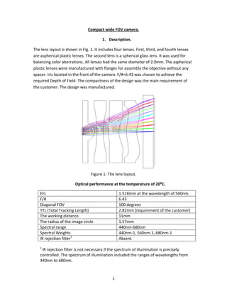
The lens layout is shown in Fig. 1. It includes four lenses. First, third, and fourth lenses
are aspherical plastic lenses. The second lens is a spherical glass lens. It was used for
balancing color aberrations. All lenses had the same diameter of 2.9mm. The aspherical
plastic lenses were manufactured with flanges for assembly the objective without any
spacer. Iris located in the front of the camera. F/#=6.43 was chosen to achieve the
required Depth of Field. The compactness of the design was the main requirement of
the customer. The design was manufactured.
Figure 1: The lens layout.
Optical performance at the temperature of 20ºC.
EFL 1.518mm at the wavelength of 560nm.
F/# 6.43
Diagonal FOV 100 degrees
TTL (Total Tracking Length) 2.82mm (requirement of the customer)
The working distance 11mm
The radius of the image circle 1.57mm
Spectral range 440nm-680nm
Spectral Weights 440nm-1, 560nm-1, 680nm-1
IR rejection filter1
Absent
1
IR rejection filter is not necessary if the spectrum of illumination is precisely
controlled. The spectrum of illumination included the ranges of wavelengths from
440nm to 680nm.

2. 2
1. MTF at the working distance of 11mm is shown in Fig. 2.
Figure 2: MTF.
2. The lateral color at the working distance of 11mm is shown in Fig. 3.
Figure 3: The lateral color.

3. 3
3. The spot diagram at the working distance of 11mm is shown in Fig. 4.
Figure 4: The spot diagram.
4. The curvature of field at the working distance of 11mm is shown in Fig. 5.
Figure 5: The curvature of field.

4. 4
5. The distortion at the working distance of 11mm is shown in Fig. 6. The maximum
distortion is 30.626%.
Figure 6: The distortion.
6. The relative illumination at the working distance of 11mm is shown in Fig. 7.
Figure 7: The relative illumination.

5. 5
7. Graph of incident ray angles versus image heights at the working distance of
11mm is shown in Fig. 8.
Figure 8: Graph of incident ray angles versus image heights.
Table 1 compares the values of CMOS CRA with incident ray angles at different image
heights (at the working distance of 11mm).
The angle of
view of the
camera in
degrees.
Height of
incident chief ray
in image surface
in mm.
Value of incident ray
angle at different
image height in
degrees.
CMOS CRA in
degrees.
Difference
between incident
ray angle and
CMOS CRA in
degrees.
5 0.123 4.24 5 -0.76
10 0.248 8.58 8 +0.58
15 0.38 13.16 14 -0.84
20 0.505 17.51 18 -0.49
25 0.667 22.94 23 -0.06
30 0.826 27.57 27.5 +0.07
35 0.991 30.83 30.5 +0.33
40 1.159 32.5 32.5 0
45 1.336 32.85 33 -0.15
50 1.57 32.48 32.3 +0.18
Table 1: Comparison of CMOS CRA and incident ray angles.

6. 6
2. Thermal sensitivity analysis.
The thermal sensitivity analysis was done according to the instructions available in the
article "HowtoModelThermalEffectsUsing Zemax". Muti-configuration editor that include
all parameters of optics changing with temperature was generated for the following
temperatures: 15°C, 20°C, 25°C, 30°C, and 35°C. The thermal sensitivity analysis was
done only at the working distance of 11mm. MTF graphs for the range of temperatures
from 15°C to 35°C are shown in Fig. 9, Fig. 10, Fig. 11, Fig. 12, and Fig. 13.
Figure 9: The MTF graph at the temperature of 15°C.
Figure 10: The MTF graph at the temperature of 20°C.

7. 7
Figure 11: The MTF graph at the temperature of 25°C.
Figure 12: The MTF graph at the temperature of 30°C.
It is clear from the figures that MTF graphs change very slightly at the range of
temperatures. The same method can be used for completing thermal sensitivity analysis
of any other parameter of optics like EFL, Magnification, and Distortion.

8. 8
Figure 13: MTF graph at the temperature of 35°C.
3. Ghost image analysis
Ghost image analysis was done by the analysis of double bouncing rays falling on the
image plane. The case of the closest focus of the ghost image to the image plane was
found. The case included the first reflection from surface 6 and the second reflection
from surface 5. The case is shown in Fig. 14 and Fig. 15. The spot diagram on the image
plane is shown in Fig. 16. MTF graph is shown in Fig. 17. So, the surface 5 and 6 should
be coated by the best anti-reflection coating to reduce irradiance of the ghost image
below the value of 0.0001* average value of irradiance of a real image.
Figure 14: Double bouncing from surfaces 6 and 5.

9. 9
Figure 15: Double bouncing from surfaces 6 and 5 (magnified picture).
Figure 16: Spot diagram obtained on the image plane.
Surface 5 Surface 6

10. 10
Figure 17: MTF graph of a ghost image.
4. Tolerance analysis.
I recommend producing the first lens by Single Point Diamond Turning (SPDT). The
tolerances of the first lens influence optical performance stronger than the tolerances of
other lenses. SPDT provides a smaller tolerance to a lateral shift of aspheric surface
(TEDX) than injection molding. Tolerance of surface irregularity (TEZI) provided by SPDT
is lower than TEZI provided by injection molding. The two tolerances located at the top
of the list of the worst offenders of MTF. See Fig. 20. Third and fourth plastic lenses can
be produced by injection molding. SPDT can be more expensive in mass production than
injection molding.
The first plastic lens had the following tolerances:
1. Tolerance to the radius of curvature TFRN was +/-2 fringes.
2. Tolerance to the thickness of the lens TTHI was +/-0.01mm.
3. Tolerance to the distance of 50µm TTHI between the iris and the front surface of
the first lens was +/-0.01mm.
4. Tolerance to shift of surface of the lens in XY plane TEDX, TEDY was +/-0.007mm.
5. Tolerance to shift of lens in XY plane TEDX, TEDY was +/-0.01mm.
6. Tolerance to the tilt of lens TETX, TETY was +/-0.1 degree.
7. Tolerance to the tilt of surface of the lens TETX, TETY was +/-0.1 degree.
8. Tolerance to surface irregularity TEZI: RMS surface irregularity was +/-
0.0001mm.
9. Tolerance to index of refraction TIND was 0.001.
10. Tolerance to Abbe number TABB was 1%.

11. 11
The spherical glass lens had the following tolerances:
1. Tolerance to the radius of curvature TFRN was +/-3 fringes.
2. Tolerance to surface irregularity TIRR was +/-1 fringe.
3. Tolerance to wedge on every side of the lens was 5 arcmin.
4. Tolerance to the thickness of the lens TTHI was +/-0.02mm.
5. Tolerance to index of refraction TIND was 0.001.
6. Tolerance to Abbe number TABB was 1%.
Third and Fourth plastic lenses had the following tolerances:
1. Tolerance to the radius of curvature TFRN was +/-2 fringes.
2. Tolerance to the thickness of the lens TTHI was +/-0.02mm.
3. Tolerance to shift of surface of the lens in XY plane TEDX, TEDY was +/-0.01mm.
4. Tolerance to shift of lens in XY plane TEDX, TEDY was +/-0.01mm.
5. Tolerance to the tilt of the lens TETX, TETY was +/-0.1 degree.
6. Tolerance to the tilt of surface of the lens TETX, TETY was +/-0.1 degree.
7. Tolerance to surface irregularity TEZI: RMS surface irregularity was +/-
0.0003mm.
8. Tolerance to index of refraction TIND was 0.001.
9. Tolerance to Abbe number TABB was 1%.
The compensator was the central thickness between the back surface of the fourth
plastic lens and the front surface of CMOS's cover glass. This thickness of 0.246mm was
adjusted in the range of +/-0.07mm for the best MTF. The minimal distance between
the plastic lens and the cover glass was 0.13mm (see Fig.1). So, the adjustment could
not lead to contact of the plastic lens with the cover glass. Tolerance to the thickness of
iris 0.05mm was 0,+0.05mm (see Fig. 18).
Figure 18: Thickness of iris and tolerances.

12. 12
I used the three angles of view of 0, 20, 40 degrees along -X,+X,-Y,+Y optical axes. See
Fig. 19. First, a sensitivity analysis was completed. The value of average MTF (sagittal
and tangential) at the spatial frequency of 80 lp/mm over the fields shown in Fig. 19 was
used as a criterion. ZEMAX calculated the 20 worst offenders of the MTF value that are
shown in Fig. 20.
Figure 19: Angles of view used in the tolerance analysis.
Type Surf 1 Surf 2 Value Criterion Change
TEDY 3 3 -0.00700000 0.51795961 -0.05163748
TEDY 3 3 0.00700000 0.51795961 -0.05163748
TEDX 3 3 -0.00700000 0.51795967 -0.05163742
TEDX 3 3 0.00700000 0.51795967 -0.05163742
TEDY 4 4 0.00700000 0.51869519 -0.05090190
TEDY 4 4 -0.00700000 0.51869519 -0.05090190
TEDX 4 4 0.00700000 0.51869599 -0.05090110
TEDX 4 4 -0.00700000 0.51869599 -0.05090110
TTHI 1 1 0.05000000 0.53931837 -0.03027872
TEZI 3 -0.00010000 0.54230915 -0.02728794
TEZI 3 0.00010000 0.54503940 -0.02455769
TTHI 4 4 -0.02000000 0.54778047 -0.02181662
TEDY 8 8 0.01000000 0.55138485 -0.01821224
TEDY 8 8 -0.01000000 0.55138485 -0.01821224
TEDX 8 8 0.01000000 0.55138536 -0.01821173
TEDX 8 8 -0.01000000 0.55138536 -0.01821173
TEDY 7 7 -0.01000000 0.55273595 -0.01686114
TEDY 7 7 0.01000000 0.55273595 -0.01686114
TEDX 7 7 -0.01000000 0.55273676 -0.01686033
TEDX 7 7 0.01000000 0.55273676 -0.01686033
Figure 20: The worst tolerance offenders of the MTF value.

13. 13
Estimated performance changes of the average MTF value based upon Root-Sum-
Square method:
Nominal MTF: 0.56959709
Estimated change: -0.11757624
Estimated MTF: 0.45202085
After that, 10 ZEMAX files with random tolerances were generated. The worst and best
MTF graphs are shown in Fig. 21, and Fig. 22 correspondingly.
Figure 21: The best MTF.
Figure 22: The worst MTF.

14. 14
Next, the analysis predicting a yield of production was completed. It is known in the
literature as Monte-Carlo analysis. The average values of MTF (sagittal and tangential) at
the spatial frequency of 80 lp/mm over the fields shown in Fig. 19 were calculated in
100 ZEMAX files. Statistic of the yield was the following:
90% > 0.33972861
80% > 0.37292765
50% > 0.39633275
20% > 0.43449065
10% > 0.44322473
5. Acknowledgments.
Mark Gokhler, Ph.D., completed the design. He provides optical design and consulting
services. Please see the website: http://www.mark-electro-optics.com. He thanks the
customer for permission to disclose the design. Application of the camera, name of the
customer, and numerical data of lens parameters cannot be disclosed according to the
requirements of the customer.