1. Predicting the Space-Time Distribution of Atlantic Seabirds
Graduate Student Researcher: Marjean Pobuda Professors: Dr. Earvin Balderama, Dr. Gregory Matthews
Department of Mathematics and Statistics, Loyola University, Chicago, IL
Motivation
Interest in developing wind resources in the offshore waters of the Mid-Atlantic
and New England has made it essential to understand characteristics of marine
bird species.
The Marine-life Data Analysis Team (MDAT) has developed models about the
distribution, abundance, and spatio-temporal variability to identify sensitive and
high-use areas in need of protection.
In the MDAT analysis, a double-hurdle model was used with a negative binomial
component to fit the typical non-zero count values of the data. In contrast, our
work employs the Poisson distribution.
Marine Bird Data Collection
The Avian Compendium housed by the National Oceanographic and Atmospheric
Administration (NOAA) provided results from 43,701 separate marine bird data
collection efforts which, in total, observed 150 different marine bird species.
Observations were grouped by calendar month which resulted in
15, 984x101 = 1, 614, 384 space-time grid cells that made up the spatial domain
for the data.
Due to repetition in the data over various cells, total amount of survey effort was
factored into the analysis.
Species with at least 200 total sightings were individually modeled.
Left to right, Roseate Tern, Northern Gannet, Herring Gull,
Wilson’s Storm-Petrel
Marine Bird Data Distributions
Count data is a statistical data type that consists of positive integers. The data
utilized in our analysis is count data for marine birds which possessed several
unique characteristics.
Zero-Inflated: Data that is zero-inflated consists of a large number of zero
observations. In histograms for the Greater Shearwater, Northern Gannet, and
Herring Gull species it is impossible to see the full range of data due to the
large number of zero counts.
Zero Inflation − Greater Shearwater Species
Counts
Frequency
0 200 400 600 800
02000400060008000100001200014000
Zero Inflation − Northern Gannet Species
Counts
Frequency
0 500 1000 1500
02000400060008000100001200014000
Zero Inflation − Herring Gull Species
Counts
Frequency
0 200 400 600 800 1000 1200
02000400060008000100001200014000
Overdispersion: Data that is overdispersed has greater variability of
observations than expected under an assumed distribution. For the species
above, histograms of all counts ≥ 50 possess extremely long tails; indicative of
the wide spread of data.
Overdispersion − Greater Shearwater Species
Counts
Frequency
0 200 400 600 800 1000
020406080
Overdispersion − Northern Gannet Species
Counts
Frequency
0 500 1000 1500
05101520253035
Overdispersion − Herring Gull Species
Counts
Frequency
0 200 400 600 800 1000 1200 1400
051015202530
Marine Bird Density Maps
The parameter estimates produced from the Bayesian hierarchical framework are
classified by month and averaged to produce monthly density maps of probability
estimates for observing a bird count greater than zero for a particular species.
These maps can be summarized further, by taking the median of all parameter
estimates in order to find the probability of observing a particular marine bird
species throughout the year.
To create density maps for the probability of observing larger counts of birds, a
threshold value can be chosen and set to produce more meaningful maps.
Examples of such maps are found below for three species with respective
thresholds of 6, 6, and 8.
Yearly Density Maps
P(y ≥ 6)
50th
percentile35.0
37.5
40.0
42.5
−76 −72 −68 −64
Longitude
Latitude
0.00
0.25
0.50
0.75
1.00
Wilson's Storm−Petrel
P(y ≥ 6)
50th
percentile35.0
37.5
40.0
42.5
−76 −72 −68 −64
Longitude
Latitude
0.00
0.25
0.50
0.75
1.00
Northern Gannet
P(y ≥ 8)
50th
percentile35.0
37.5
40.0
42.5
−76 −72 −68 −64
Longitude
Latitude
0.00
0.25
0.50
0.75
1.00
Herring Gull
To examine the variability of our yearly estimates above, the 5th
and 95th
percentile are constructed. By subtracting these two estimates the density maps
below confirm that our model’s uncertainty is small.
Difference of Variability Maps
P(y ≥ 6)
95th
− 5th
percentile35.0
37.5
40.0
42.5
−76 −72 −68 −64
Longitude
Latitude
0.0
0.1
0.2
Wilson's Storm−Petrel
P(y ≥ 6)
95th
− 5th
percentile35.0
37.5
40.0
42.5
−76 −72 −68 −64
Longitude
Latitude
0.0
0.1
0.2
Northern Gannet
P(y ≥ 8)
95th
− 5th
percentile35.0
37.5
40.0
42.5
−76 −72 −68 −64
Longitude
Latitude
0.0
0.1
0.2
Herring Gull
For species of interest, the 5th
and 95th
variability maps along with the yearly
density map can be compared to detect favored habitats. This information could
potentially aid future wind-resource location planning.
Yearly Density Map and Variability Percentile Maps
P(y ≥ 1)
5th
percentile35.0
37.5
40.0
42.5
−76 −72 −68 −64
Longitude
Latitude
0.00
0.25
0.50
0.75
1.00
Roseate Tern
P(y ≥ 1)
50th
percentile35.0
37.5
40.0
42.5
−76 −72 −68 −64
Longitude
Latitude
0.00
0.25
0.50
0.75
1.00
Roseate Tern
P(y ≥ 1)
95th
percentile35.0
37.5
40.0
42.5
−76 −72 −68 −64
Longitude
Latitude
0.00
0.25
0.50
0.75
1.00
Roseate Tern
Negative Binomial vs. Poisson Distribution
One of the main motivations behind selecting our research topic was to analyze
the marine bird data using a double-hurdle model with a Poisson component for
the typical non-zero counts. There are several reasons for this choice.
Benefit: The estimation of one less parameter. A key characteristic of the
Poisson distribution is that its mean is equal to its variance therefore only one
parameter is needed.
Benefit: Interpretability. For count data, the Poisson distribution is the standard
choice in the field and as such, the meaning of our results is easily understood.
Methods
Bayesian Hierarchical Framework:
Bayesian Inference
Given the zero-inflation and overdispersion in our data, selecting an
appropriate prior distribution is challenging.
A double hurdle model is selected so we can split our likelihood function into
three pieces: one for the zero counts, a Poisson for the typical counts, and a
generalized Pareto for the extreme counts.
Likelihood Function:
p(y) =
θ1 for y = 0
(1 − θ1) ∗ (1 − θ2) ∗ f (y|λ) for 1 ≤ y < threshold
(1 − θ1) ∗ θ2 ∗ g(y|µ, σ, ξ) for y ≥ threshold
The Metropolis-Hastings Algorithm
A Markov chain Monte Carlo (MCMC) is a method for obtaining a sequence
of random samples from a distribution when the shape of the distribution is
unknown.
We run the MCMC over our likelihood function to obtain an approximation
of our distribution for each of the three likelihood pieces.
Assessing Model Convergence:
As the MCMC algorithm runs over the course of 100, 000+ iterations, we can
monitor the current values for each parameter estimate and observe the
likelihood function.
Convergence occurs when the MCMC algorithm stabilizes and start to
consistently fluctuate around the same value.
Constructing Maps
The density maps are created in R with packages ggmap() and ggplot2().
Through ggmap() we can download maps from Google Earth, plot them in
layers and then use ggplot2() to plot additional content layers with our model
output on top of the maps.
Conclusions
Able to estimate parameters for 7 covariates with Bayesian regression to predict
the space-time distribution of 5 marine bird species.
The habitat trends of marine birds identified through map patterns.
Model’s uncertainty of parameter estimates is small.
Future Considerations
Compare density maps with those from the MDAT study.
Extend density map modeling to additional marine bird species.
mpobuda@luc.edu