A Guide to SPSS Statistics
•
2 likes•1,238 views

Handy guide for SPSS stats info, bit old but still useful

Recommended
More Related Content
What's hot
What's hot (20)
Similar to A Guide to SPSS Statistics
Similar to A Guide to SPSS Statistics (20)
More from Luke Farrell
More from Luke Farrell (14)
Recently uploaded
Recently uploaded (20)
A Guide to SPSS Statistics
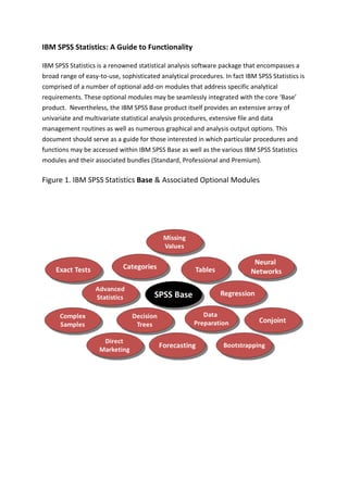
- 1. IBM SPSS Statistics: A Guide to Functionality IBM SPSS Statistics is a renowned statistical analysis software package that encompasses a broad range of easy-to-use, sophisticated analytical procedures. In fact IBM SPSS Statistics is comprised of a number of optional add-on modules that address specific analytical requirements. These optional modules may be seamlessly integrated with the core ‘Base’ product. Nevertheless, the IBM SPSS Base product itself provides an extensive array of univariate and multivariate statistical analysis procedures, extensive file and data management routines as well as numerous graphical and analysis output options. This document should serve as a guide for those interested in which particular procedures and functions may be accessed within IBM SPSS Base as well as the various IBM SPSS Statistics modules and their associated bundles (Standard, Professional and Premium). Figure 1. IBM SPSS Statistics Base & Associated Optional Modules
- 2. IBM SPSS Statistics Base – Analytical Procedures As a general overview of the analytical functionality within IBM SPSS Base, the following procedures all appear as menu items within the core product. • Reports – This menu item contains procedures for creating a wide range of summary and listing reports. • Descriptive Statistics – This includes an extensive range of descriptive statistical functions including frequency tables, crosstabs and the Explore procedure which generates histograms, boxplots and confidence intervals. • Compare Means - Generates Means comparison tables as well as parametric T-Tests and one-way ANOVA. • Correlate - Includes Bivariate Correlations (Pearson and Spearman) and Partial Correlation procedures. • Regression - includes the Automatic Linear Models procedure as well as Linear Regression, Curve Estimation, Partial Least Squares and Ordinal regression. • Classify - Includes three clustering methods (Two Step, K-Means, and Hierarchical) also includes Discriminant function analysis. • Data Reduction - Includes Principal Component Analysis and Factor Analysis. • Scale - Contains functions to perform Reliability analysis and Multi-Dimensional Scaling (ALSCAL). • Non-Parametric Tests - Contains a range of Non-Parametric tests for one sample, independent samples and related samples. • Simulation – This procedure allows users to create data that can be applied to existing models or entered manually as equations. • Time Series - Provides a number of descriptive time series procedures including sequence charts and auto correlations. • Multiple Response - Allows users to define multiple response sets for frequency and cross-tabulation analysis. • Quality Control - Includes Control charts and Pareto charts. The following section provides more detailed information relating to the analytical procedures found within IBM SPSS Base.
- 3. Reports Menu • Used for creating listing reports similar to those produced by database software • Can list values for individual cases or summary statistics broken down by a grouping variable • OLAP Cubes are used to produce layered reports which users can ‘drill down’ into via the Output Viewer • Often used for financial reports • Both Report Summaries in Columns and Report Summaries in Rows produce plain text output rather than the normal SPSS formatted text output Descriptive Statistics Menu • Frequencies and Descriptives are used to summarise individual variables (categorical and continuous respectively) • The Explore procedure provides a large collection of statistical and graphical routines for examining distributions including histograms, m-estimators, Box plots and Stem and Leaf plots • Crosstabs is one of the most widely used procedures to examine the relationship between categorical variables. The procedure also contains a number of statistical tests and association measures • TURF (Total Reach and Frequency) analysis is a procedure used for providing estimates of media or market potential and devising optimal communication and placement strategies given limited resources. TURF analysis identifies the number of users reached by a communication, and how often they are reached. • Ratio provides a comprehensive list of summary statistics for describing the ratio between two scale variables. Often used in analysing real estate data to investigate the ratio of valuations to actual selling price • PP and QQ plots are generally used to evaluate whether or not the distribution of a variable matches a given distribution (e.g. normal, laplace, logistic, lognormal etc.) Compare Means Menu • The Means procedure provides reports of summary statistics (not just averages) broken down by independent grouping variables. It is a flexible procedure that also includes tests for linearity and eta values
- 4. • The One-Sample T-Test is a parametric procedure that tests whether the mean of a single variable differs from a specified target value. • The Independent-Samples T-Test is a classic statistical procedure to compare the means for two groups of cases • The Paired-Samples T-Test procedure compares the means of two variables for a single group. Often used to examine differences in before and after situations • The One-Way ANOVA procedure provides the ability to test for significant differences between more than two groups (i.e. k groups). It also allows users to identify where the actual differences are using an extensive range post-hoc tests Correlate Menu • The Bivariate Correlation procedure provides both parametric and non-parametric measures of association between variables. Correlation coefficients are widely used to identify the strength of the linear relationships between pairs of variables • The Partial Correlations procedure computes partial correlation coefficients that describe the linear relationship between two variables while controlling for the effects of one or more additional variables • Examples of this might include examining the relationship between crime rates and average property value but controlling for unemployment levels. This would allow us to test whether or not any apparent relationship between crime and property value existed irrespective of the local unemployment rate. • The Distance measure calculates a wide variety of statistics measuring either similarities or dissimilarities (distances) either between pairs of variables or between pairs of cases. It is often used as a supporting exploratory procedure for techniques such as cluster or factor analysis Regression Menu • Automatic Linear Models is a procedure that enables automatic model selection and data preparation for estimating the values of a continuous target field. The procedure also allows users to invoke ‘bagging’ routines to create ensemble models with an emphasis on maximising model stability or alternatively ‘boosting’ routines to create ensemble models that are focussed on estimation accuracy. • The Linear Regression procedure is the all-time classic predictive algorithm. This procedure supports multiple linear regression with a number of stepwise procedures and fit measures. Classic examples include building predictive models to estimate sales based on advertising spend, discount values, competitor price etc.
- 5. • The Curve Estimation procedure produces estimation statistics and related plots for 11 different types of curve. This allows users to investigate the most appropriate curvilinear fit between variables. • Partial Least Squares is a predictive technique that is an alternative to, for example, ordinary least squares (OLS) regression and it is particularly useful when predictor variables are highly correlated. PLS combines features of principal components analysis and multiple regression. Note however that PLS is an extension command that requires the IBM SPSS Statistics - Integration Plug-in for Python to be installed on the system where you plan to run PLS. • The PLS Extension Module must be installed separately, and can be downloaded from http://www.ibm.com/developerworks/spssdevcentral Classify Menu • Two-Step Cluster reveals natural groupings (or clusters) within a dataset that would otherwise not be apparent. The Two-Step procedure allows the use of both categorical and continuous fields, is highly scalable and can automatically select the number of clusters. • K-Means Cluster (otherwise known as Quick Cluster) is a relatively fast and simple cluster technique that requires continuous (or dichotomous) data in order to effectively group cases together. K-Means also requires that the number of clusters to be created is specified beforehand. • Hierarchical Cluster Analysis also attempts to group similar cases together in order to create clusters. As with K-Means, the number of clusters must be specified beforehand and the data should be continuous (or dichotomous). Hierarchical Cluster is a resource-intensive procedure that requires a distance matrix to be computed in the background showing the distance between every single. As such, although it is possible to follow the clustering process in detail, this technique is generally used with small datasets. • Discriminant Analysis can be used to build a predictive model for different groups. It uses linear combinations of continuous predictor fields in order to create discriminant functions. Examples might include building a predictive model to estimate which of three tariffs subscribers to a new mobile phone service will sign up to based on their age, income level, previous history of phone usage and size of family.
- 6. Dimension Reduction Menu • The Dimension Reduction menu offers both Factor Analysis and Principal Components Analysis (PCA) as tools to uncover the underlying factors that explain correlations in a set of variables. • Factor Analysis and PCA allow analysts to distil the factors that underpin a number of correlated variables. Examples of Factor Analysis include examining the underlying factors that drive customer satisfaction. In such an example, factor analysis could identify the top four composite factors when respondents have been asked to rate the performance of a company using 30 different rating scales. • The factor analysis procedure offers a high degree of flexibility: – Seven methods of factor extraction – Five methods of rotation – Three methods of computing factor scores Scale Menu • Reliability Analysis measures the consistency of a set of measurements or a given ‘measuring instrument’. This can take the form of assessing the degree to which scales or instruments provide consistent results over time or whether two independent assessors give similar scores (known as inter-rater reliability). • Multidimensional Scaling (ALSCAL) attempts to find the structure in a set of distance measures between objects or cases. This task is accomplished by assigning observations to specific locations in a conceptual space (usually two or three- dimensional) such that the distances between points in the space match the given dissimilarities as closely as possible. In many cases, the dimensions of this conceptual space can be interpreted and used to further understand your data. • A wider range of scaling techniques is available in the IBM SPSS Categories module. Non Parametric Tests Menu • The Non-Parametric Tests menu contains a collection of tests designed for situations where, for example, the test data does not sufficiently meet the requirements of many classical statistical tests. • Example situations include comparing values from two distributions that are not normally distributed or which are based on rank order values (such as rating scales).
- 7. • The tests that are available in these dialogs can be grouped into three broad categories based on how the data are organized: – A one-sample test analyses one field. – A test for related samples compares two or more fields for the same set of cases. – An independent-samples test analyses one field that is grouped by categories of another field. • The Non-Parametric Tests procedure also includes access to a number of legacy dialogs that allow direct access to a host of popular non-parametric procedures including: – Mann-Whitney U (two independent samples) – Kruskall-Wallace H ( more than two independent samples) – Wilcoxon signed-rank and McNemar tests (two related samples) – Friedman (more than two related samples) Simulation Menu • Simulation allows users to examine ‘what if’ scenarios by testing the effect of changing the values of key inputs in a predictive model. For example, if you have a response model that includes advertising spend as an input, you can use the simulation procedure to model the effect of reducing or increasing the advertising spend to determine how the response rate changes. • Simulation in IBM SPSS Statistics uses the Monte Carlo method. Uncertain inputs are modeled with probability distributions (such as the triangular distribution), and simulated values for those inputs are generated by drawing from those distributions. Inputs whose values are known are held fixed at the known values. The predictive model is evaluated using a simulated value for each uncertain input and fixed values for the known inputs to calculate the target (or targets) of the model. The process is repeated many times (typically tens of thousands or hundreds of thousands of times), resulting in a distribution of target values that can be used to answer questions of a probabilistic nature. • To run a simulation, you need to specify details such as the predictive model, the probability distributions for the uncertain inputs, correlations between those inputs and values for any fixed inputs. Once you've specified all of the details for a simulation, you can run it and optionally save the specifications to a simulation plan file. You can share the simulation plan with other users, who can then run the simulation without needing to understand the details of how it was created.
- 8. Time Series Menu • The Sequence Charts procedure provides simple, exploratory line charts for time- based data. It allows different sequences of values to be illustrated and compared and offers some basic transformation functions (natural log, difference and seasonal difference) • Auto Correlations is an exploratory procedure which returns auto correlation and partial autocorrelation information in the form of statistics and charts including transformation functions such as natural log, difference and seasonal difference. • Auto Correlations are useful for finding repeating patterns in a sequence. They in effect, measure the degree to which the preceding values correlate with subsequent values and as such are useful in exploring Time Series data. • Cross Correlations are used when measuring information between two different time series. They return information that show how strongly related the sequences are to each other across a timeframe. Cross Correlations are a useful exploratory procedure in Time Series when analysts wish to identify sequences or series which are good predictors of each other. Multiple Response Menu • The Multiple Response procedure is used to analyse data where the categories are not mutually exclusive. Examples of this include asking respondents in a questionnaire to ‘Please tick all that apply’ or when analysing where customers made purchases from 40 different products groups. • The Multiple Response procedure requires users to define a multiple response set: that is, they must identify all the variables that record the non-mutually exclusive selections and save them as a set. • Users can then include the newly defined multiple response set in special multiple response frequencies and crosstabs procedures which are found under the Multiple Response menu. Note that: • Using this particular procedure means that Multiple Response sets cannot be saved and must be redefined each time a new session is started. • Furthermore, the Multiple Response procedure within SPSS Statistics Base is independent of the Multiple Response procedure in the IBM SPSS Tables module (where sets may be saved for re-use).
- 9. • In SPSS Statistics Base, the Multiple Response procedure does not contain any statistical tests. Quality Control • The Quality Control menu contains two charting techniques: Control Charts and Pareto Charts. Both of these chart types are often used in quality control applications to monitor or investigate changes in quality and to identify the main causes of change. • Control charts are used to determine whether a manufacturing or business process is in a state of statistical control or not. A control chart is a specific kind of graph that monitors a process over time with a view to identifying significant change to the process rather than just natural variability. • Pareto charts are specific types of bar chart used in quality control situations. The purpose of the chart is to highlight in descending order, the main causes of defects/ quality errors/ events where a process has moved beyond the allowed control limits. The following figures illustrate which optional modules are provided with the Standard, Professional and Premium editions of IBM SPSS Statistics respectively. Figure 2. IBM SPSS Statistics Standard
- 10. Figure 3. IBM SPSS Statistics Professional Figure 4. IBM SPSS Statistics Premium