Drainage Engineering lecture note

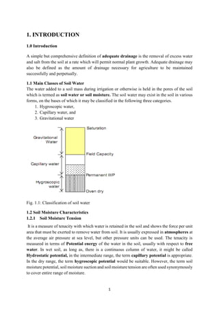
1. 1
1. INTRODUCTION
1.0 Introduction
A simple but comprehensive definition of adequate drainage is the removal of excess water
and salt from the soil at a rate which will permit normal plant growth. Adequate drainage may
also be defined as the amount of drainage necessary for agriculture to be maintained
successfully and perpetually.
1.1 Main Classes of Soil Water
The water added to a soil mass during irrigation or otherwise is held in the pores of the soil
which is termed as soil water or soil moisture. The soil water may exist in the soil in various
forms, on the bases of which it may be classified in the following three categories.
1. Hygroscopic water,
2. Capillary water, and
3. Gravitational water
Fig. 1.1: Classification of soil water
1.2 Soil Moisture Characteristics
1.2.1 Soil Moisture Tension
It is a measure of tenacity with which water is retained in the soil and shows the force per unit
area that must be exerted to remove water from soil. It is usually expressed in atmospheres at
the average air pressure at sea level, but other pressure units can be used. The tenacity is
measured in terms of Potential energy of the water in the soil, usually with respect to free
water. In wet soil, as long as, there is a continuous column of water, it might be called
Hydrostatic potential, in the intermediate range, the term capillary potential is appropriate.
In the dry range, the term hygroscopic potential would be suitable. However, the term soil
moisture potential, soil moisture suction and soil moisture tension are often used synonymously
to cover entire range of moisture.

2. 2
1.2.2 Soil Moisture Constants
Soil moisture is always subjected to pressure gradients and vapor pressure differences that
cause it to move. Thus, soil moisture cannot said to be constant at any pressure. The following
are soil moisture constants that are of particular significance in agriculture.
1. Saturation Capacity: When all pores of soil are filled with water, the soil is said to be
under saturation capacity or maximum water holding capacity. The tension at saturation
capacity is almost zero and is equal to free water surface
2. Field capacity (F.C): It is the moisture content after drainage of gravitational water
and moisture content become stable. At field capacity, the large soil pores are filled
with air, micro pores are filled with water. The field capacity is the upper limit of
available moisture range in soil and plant relations and moisture tension at field capacity
varies from soil to soil, but generally range from 1/10th to 1/3rd of atmosphere.
3. Permanent Wilting Point (PWP): It is the soil moisture content at which plants can
no longer obtain enough moisture to meet transpiration requirements, remain wilted
unless water is added to soil. The moisture tension of soil at PWP ranges from 7 to 32
atmospheres. 15 atmosphere is the pressure commonly used for this point. The
moisture content at which the wilting is complete and the plants die is called ultimate
wilting.
4. Available Water: The soil moisture between field capacity and permanent wilting
point is referred as available moisture.
Fig.1.2: Available moisture content

3. 3
Table 1.1: Range of available water holding capacity of soils
Soil type % moisture, based on dry weight of soil. Depth of available water per unit of
soil(cm per meter depth of soil)
Field Capacity Permanent WP %
Fine sand 3 -5 1 -3 2- 4
sandy loam 5 - 15 3 - 8 4 - 11
Silt loam 12 - 18 6 - 10 6 - 13
Clay loam 15 30 7 - 16 10 - 18
Clay 25 - 40 12 - 20 16 - 30
1.2.3 Soil Water Potential
Total water potential is the amount of work required per unit quantity of pure water to
transport, irreversibly and isothermally, a small quantity of water from a pool of pure water at
a specified elevation at atmospheric pressure to the soil water at the point under consideration.
Differences in potential energy of water from one point in a soil system to another give rise to
the tendency of water to flow within the soil. In the soil, water moves continuously in the
direction of decreasing potential energy.
Soil water potential can be expressed in three different units:
Remember: Potential = Force x Distance = mgl = ρwVgl (Nm)
Potential per unit mass (𝜇): 𝜇 = potential/mass = gl (Nm/kg)
Potential per unit volume (Ψ): Ψ= potential/volume =
𝜌𝑤Vgl
𝑉
= 𝜌𝑤gl (N/m2
)
Potential per unit weight (h): ℎ = 𝑝𝑜𝑡𝑒𝑛𝑡𝑖𝑎𝑙/𝑤𝑒𝑖𝑔ℎ𝑡 = 𝑚𝑔𝑙 / 𝑚𝑔 = 𝑙 (m, head unit) =
equivalent height of water.
Consequently, we do not need to compute the soil-water potential directly by computing the
amount of work needed, but measure the soil water potential indirectly from pressure or water
height measurements.
Water potential is more easily understood if we break it down into component potentials. For
water potential, Ψ𝑤 we can write Ψ𝑤 = Ψ𝑝 + Ψ𝑠 + Ψ𝑚 (1.1)
Where Ψ𝑤= water potential, = Ψ𝑝 pressure potential, =Ψ𝑠 solute potential and Ψ𝑚= matric
potential, We can also define, a gravitational potential,Ψ𝑧 which when combined with the water
potential, Ψ𝑤 gives the total potential, Ψ𝑡
Ψ𝑡=Ψ𝑤+Ψ𝑧 (1.2)
If we are concerned only with liquid water, the flow in the soil, the solute component is
essentially zero. If there are no semi permeable membranes,
Ψ𝑡=Ψℎ=Ψ𝑧+Ψ𝑚+ Ψ𝑝 (1.3)
1.2.3.1 Gravitational Potential
Weight is one of the most convenient methods of specifying the unit of water. In this case, the
gravitational potential (𝚿𝒛) is the difference in elevation of the point in question and the
reference point. If the point in question is above the reference point, Ψ𝑧 is positive; if the point
in question is below the reference, Ψ𝑧 is negative.

4. 4
In Figure 1.4, two points in a soil are located at a specific distance from a reference point Z.
Gravitational potential of point A is 6 inches and of point B is 4 inches, thus the difference in
gravitational potential between the two points is 6 inches - (-4 inches) = 10 inches.
Fig. 1.4: Gravitational potential
1.2.3.2 Matric Potential
When the unit quantity of water is expressed as weight, then, Ψ𝑚 is the vertical distance
between the measured point of the soil (ceramic cup of Figure 1.5 a) and the water surface of
a water filled manometer. Matric potential is a dynamic soil property and will be at a
theoretical zero level for a saturated soil. The matric potential of a soil system results from
capillary and adsorptive forces due to the soil matrix. As we can see from Figure 1.5 b, a
distance z is the distance from the top of the mercury column to the center of the ceramic cup.
zHg is defined as the distance from the top of the mercury column to the surface of mercury in
the reservoir. From this, the weight matric potential, Ψ𝑚, is defined by Taylor and Ashcroft
as 𝚿𝒎 = 𝐳𝐇𝐠 ∗
𝛒𝐇𝐠
𝛒𝐰
+ 𝐳_______________________________(𝟏. 𝟒)
Where ρHg is the density of mercury (13.6 g/cm3
) and ρw is the density of water (1 g/cm3
)
∴ Ψ𝑚 = −13.6 zHg + z______________________________________(𝟏. 𝟓)
Fig. 1.5: Different types of Tensiometers: (a) a water

5. 5
manometer connected to a ceramic cup installed in soil at the designated depth, Ψm equals −h;
(b) a mercury manometer connected to a ceramic cup installed in soil at the desired depth,
𝛹𝑚 = −𝑧𝐻𝑔 × 13.6 + 𝑍; and (c) a vaccum gauge tensiometer, 𝛹𝑚 = −34 × 10 𝑐𝑚 +
100 𝑐𝑚 = −240 𝑐𝑚.
1.2.3.3 Pressure Potential
The pressure potential applies mostly to saturated soils. When water quantity is expressed as
a weight, pressure potential is the vertical distance between the water surface and a specified
point.
1.2.3.4 Osmotic Potential
Osmotic potential is due to the presence of solutes in soil moisture that affect its
thermodynamic properties (e.g., free energy). Presence of solutes in soil lowers the vapor
pressure of soil moisture and affects its Ψ𝑠. The Ψ𝑠 refers to the change in energy per unit
volume of water when solutes identical in composition to the soil solution at the point of interest
in the soil are added to pure, free water at the elevation of the soil.
1.3 Water flow in Soils
If piezometers and tensiometers installed in a soil register different heads of water at different
positions, water moves from positions where the head is high to those where it is low.
1.3.1 Darcy’s Law – saturated soils
In 1856 Darcy published the results of experiments on water flow down columns of sand. These
showed that the rate of flow Q was directly proportional to the head difference,∆ℎ causing the
flow and the cross-sectional area A of the column, and inversely proportional to its length L.
Thus:Q = KA
∆h
L
(1.6)
Fig. 1.8: Darcy’s law

6. 6
The proportionality constant k in eqn. 1.6 has units of velocity and is known as the hydraulic
conductivity of the porous material. Equation 1.6 is Darcy's law, which can be written in
terms of the flow velocity v per unit area as: 𝑣 = −
K∆H
L
________(1.7)
The negative sign in eqn. 1.7 shows that the flow is in the direction of decreasing head. Since
with flow in saturated non-shrinking soils there can be no increase or decrease of water content:
𝑑𝑖𝑣 𝑣 = 0 and since k in such soils is a constant: ∇2
ℎ = 0________(1.8)
Which is Laplace's equation. Equation 1.8 can be used to obtain distributions of h with given
boundary conditions and then equation 1.7 is used to obtain the flow pattern.
1.3.2 Richard’s equation-unsaturated soils
Richards (1931) argued that the flow of water in unsaturated soils was similar to that in
saturated soils except that there were fewer conducting pores. Thus Darcy's law would be
obeyed with a hydraulic conductivity value greatly reduced because of the absence of the larger
pores that empty first. Richards also recognized that the wetting and draining of the soils
provide a component of flow. In an inert porous material that does not swell and shrink:
𝜕𝜃
𝜕𝑡
= −𝑑𝑖𝑣 𝑣 (1.9)
Where 𝜃 = volumetric moisture content. Since v is given by Darcy's law (eqn. 1.7), it follows
that:
∂θ
∂t
= div (
K∆H
L
) = div (
K∆P
L
) +
∂k
∂z
(1.10)
Where k is now the hydraulic conductivity of the unsaturated soil. Equation 1.10 is a form of
the equation derived by Richards. In this equation the relationship between 𝜃 and p is given
by the moisture characteristic: the hydraulic conductivity k decreases rapidly as the soil
desaturates, and can be given as a function of either 𝜃 or p; the k (𝜃) function shows little
hysteresis, whereas the k(p) function.
For steady-state conditions when 0 and h do not change with time, eqn. 1.10 becomes:
𝑑𝑖𝑣 (
K∆H
L
) = 0 (1.11)
It is seen that Laplace's equation (eqn. 1.8) is a special case of eqn. 1.11 with k a constant.
The accurate relationships between𝜃, p and k have to be given in graphical, as in Figure 1.9, or
numerical form. However, various empirical relationships for k (𝜃) and k (p) as well as those
for p (𝜃), usually for the draining relationships, are often used to facilitate solutions of
equations 1.10 and 1.11. For example, k (p) is often found to be well represented by an
exponential relationship:
𝐾(𝑝) = 𝐾𝑜𝑒𝑥𝑝(𝑐𝑝) (1.12)
Where k0 is the hydraulic conductivity of the saturated soil and c is a constant, that allows
analytical solutions to many two and three dimensional steady state problems; or a power law
relationship:
𝐾(𝑝) =
𝑎′
[1+𝑏′(−𝑝)𝑐′]
(1.13)
Where a', b' and c' are constants.
K (𝜃) is often described by: 𝐾(𝜃) = 𝐾𝑜𝜃𝑐"
(1.14)
The moisture release curve p (𝜃) is described by a simple power law equation:
𝑝(𝜃) =
𝑎"(𝜃𝑜−𝜃)𝑛
𝜃𝑚 (1.15)
where c", a", m and n are constants, and 𝜃0 is the saturated soil-water content.

7. 7
Boundary conditions
The pattern of soil water flow is determined by the values of hydraulic head that occur at the
boundaries of the given soil region, and by the soil water relationships in unsaturated soils. The
boundary values are used in solving the general flow equation (Richards' equation [eqn 1.10],
which becomes Laplace's equation [eqn 1.8] for steady groundwater flow) to obtain
distributions of p or h and𝜃, and of the flow using eqn.1.7, for a given situation.
The hydraulic head value itself may be imposed or may be the result of an imposed flux that
produces a gradient of the head h. Figure 1.10 illustrates various types of boundary conditions
involved in soil-water flow problems:
(a) On a ponded soil surface, as for ponded surface infiltration and ponded surface drainage, p
= 0 and h = 0 if the head is measured from the soil surface.
(b) For constant rate infiltration through the soil surface at a rate F that does not saturate the
soil so that p < 0, the prescribed flux gives
𝜕ℎ
𝜕𝑧
= − 𝐹 /𝑘 through the surface.
(c) At a water table there is a mixed boundary condition with p = 0 and h = z, and with the
prescribed flux V between the groundwater region and unsaturated soil-water region
giving 𝜕h/𝜕z = − 𝑉 /𝑘.
(d) On the walls of a drain installed below a water table and running full so that p =P at its top
(P > 0), p = P + d + r0 - z and h = P + d + r0, where dis the height of the drain axis and r0 is
the radius of the drain.
(e) On the walls of a drain installed below a water table but not running full, a seepage surface
where p = 0 and h = z exists above the water level. Below the water level, p = z0 - z and h
= z0, where z0 is the height of the water level.
(f) On the walls of a water-filled ditch, water seeps out of the saturated soil above the ditch-
water level at height z0 through a surface of seepage where p = 0 and h = z. Below the water
level, p = z0 - z and h = z0 .
1.4 Soil-water movement above water tables
When rainfall rates are high, water tables build up to near the surface and drains run fast. After
the cessation of such periods of heavy rainfall, water tables fall and the soil above desaturates,
and the drain discharge decreases.
When the drains finally stop running, the water table throughout is at drain level, and, provided
evaporation from the surface is negligible, the water in the unsaturated soil is in equilibrium
with the water table. The soil is then said to be at field capacity. The soil can then lose water
further through evaporation and plant use. The decrease in the amount of water held in the soil
profile below the state of field capacity is termed the soil-water deficit.
1.4.1 Steady-state flow between soil surface and water table
With steady one-dimensional vertical flow, the flow per unit area 𝑣 is given everywhere by
Darcy's law as the product of the hydraulic conductivity at the prevailing soil-water content
and the hydraulic potential gradient at the given position. Thus:
𝑣 = −𝐾
𝜕𝑝
𝜕𝑧
= −𝐾 (
𝜕ℎ
𝜕𝑧
+ 1) (1.16)

8. 8
Since at the water table p = 0, integration of eqn 1.16 gives the height above the water table, z
where the soil-water pressure has the value p:
z = − ∫
dp
1+𝑣
k(p)
⁄
p
0
(1.17)
This can be integrated numerically for any k (p) relationship, or analytically if k (p) is given in
a simple algebraic form such as eqn. 1.12. For a steady-state rainfall rate (𝑣 negative), this
gives soil-water pressures and soil-water contents that approach constant values as the height
above the water table becomes large, as illustrated in Figure 1.11(a); the constant values are
those corresponding to a hydraulic conductivity equal to the steady rainfall rate.
When there is no flow so that the profile is at field capacity, with 𝑣 = 0 in eqn. 1.17, z = − p
everywhere. Thus the profile corresponds to the moisture characteristic curve. With steady
upward flow, often termed capillary rise, from a water table to the soil surface where it is
removed by plant use or evaporation (𝑣 positive), the profiles are below field capacity. In this
case there is a maximum flow rate 𝑣1 that can be sustained for a given depth of water table
below the soil surface before the soil-water pressure approaches a large negative value and the
soil properties, rather than meteorological conditions, limit the capillary rise. The depth Z for
which the soil becomes limiting for the flux 𝑣1 is:
z = − ∫
dp
1+
𝑣1
k(p)
⁄
∞
0
(1.18)
The dependence of the limiting evaporation rate on the depth Z for a silt soil is shown in Figure
1.11(b). Since evaporation rates produced by meteorological conditions rarely exceed 10
mm/d, soil conditions do not limit the evaporation unless the water table is deeper than about
1 m below the soil surface.
1.4.2 Non-steady-state flow to water tables
Any changes in the boundary conditions at the soil surface produce non-steady-state soil-water
flow. Such changes have an effect on the flux interchange between the unsaturated soil-water
and groundwater regions.
Since the extent of the groundwater region depends on this flux, the water table position does
not remain constant as a result of such changes. Accurate simulations can be made using
numerical procedures to solve
𝜕𝜃
𝜕𝑡
=
𝜕
𝜕𝑧
(𝑘
𝜕𝑝
𝜕𝑧
) +
𝜕𝑝
𝜕𝑧
.
However, using approximations based on the concept of specific yield, the water table
movement can be more simply computed as a result of changing meteorological conditions,
with the non-steady-state profiles assumed to be a succession of average steady-state ones.

9. 9
CHAPTER TWO
DRAINAGE AND CROP PRODUCTION
2.1 THE NEED FOR DRAINAGE
When irrigation is introduced in an area, it affects the water balance. As it may be seen in
figure 2.1 to apply irrigation water to a crop, it has to be diverted from a river or lake (1) or
pumped from the groundwater reservoir (2). The amount of water needed has to be greater than
the quantity required by the crop because some of it will leave the area in various ways: not
only will it be used by the crop as evapotranspiration (3), but some of it will be lost as
evaporation (4), as seepage (5) and operational spills (6) from the irrigation canal system, as
tail water runoff from irrigated fields (7), and as deep percolation (8).
In the field, irrigation water, together with any rainfall (9), will be partly stored on the soil
surface (10) and will partly infiltrate into the soil (11). If rain or irrigation continues for long
periods, pools may form on the soil surface. This accumulation of excess water on the soil
surface is called ponded water. It needs to be removed.
Ponding is the accumulation of excess water on the soil surface.
Fig. 2.1: The water balance in an irrigated area
Part of the water that infiltrates into the soil will be stored in the soil pores and will be used by
the crop (3); another part of the water will be lost as deep percolation (8). When the percolating
water reaches that part of the soil which is saturated with water, it will cause the water table to
rise (12). If the water table reaches the root zone, the plants may suffer (Figure 2.2). The soil
has become waterlogged. Drainage is needed to remove the excess water and stop the rise of
the water table.
Waterlogging is the accumulation of excess water in the root zone of the soil. Even if irrigation
water is of very good quality, it will contain some salts. So, bringing irrigation water to a field
also means bringing salts to that field. The irrigation water is used by the crop or evaporates
directly from the soil. The salts, however, are left behind (Figure 2.3).

10. 10
This process is called salinization. If these salts accumulate in the soil, they will hamper the
growth of crops.
Salinization is the accumulation of soluble salts at the soil surface, or at some point below the
soil surface, to levels that have negative effects on plant growth and/or on soils.
Fig. 2.2: After irrigation or rainfall, the water table may rise and reach the root zone
Some crops are more tolerant to salts than others (Table 2.1). Highly tolerant crops can
withstand a salt concentration up to 10 g/l in the saturation extract. Moderately tolerant crops
can withstand up to 5 g/l, and sensitive crops up to 2.5 g/l. If sensitive crops are to be grown,
drainage is needed to remove the salts.
So, drainage is used to control ponding at the soil surface, to control waterlogging in the
Soil, and to avoid salinization.
Table 2.1: Tolerance levels of some of the major crops

11. 11
Fig. 2.3: Irrigation water bring salts to the soil
Drainage is the removal of excess water and dissolved salts from the surface and subsurface
of the land in order to enhance crop growth. Drainage is needed for successful irrigated
agriculture because it controls Ponding, waterlogging and salinity.
2.2 DRAINAGE TO CONTROL PONDING
To remove ponding water from the surface of the land, surface drainage is used. Normally,
this consists of digging shallow open drains.
Surface drainage is the removal of excess water from the surface of the land by diverting it
into improved natural or constructed drains, supplemented, when necessary, by the shaping
and grading of the land surface towards such drains.
Fig. 2.4: Surface drainage to remove excess water from the land surface
2.3 DRAINAGE TO CONTROL WATERLOGGING
To remove excess water from the root zone, subsurface drainage is used (Figure 2 .5). This is
done by digging open drains or installing pipes, at depths varying from 1 to 3 m. The excess
water then flows down through the soil into these drains or pipes. In this way, the water table
can be controlled.

12. 12
Subsurface drainage is the removal of excess water and dissolved salts from soils via
groundwater flow to the drains, so that the water table and root-zone salinity are controlled.
Fig. 2.5: Subsurface drainage to control the water table and to remove excess water and
dissolved salts from the root zone
2.4 DRAINAGE TO CONTROL SALINIZATION
To remove salts from the soil, more irrigation water is applied to the field than the crops require.
This extra water infiltrates into the soil and percolates through the root zone. While the water
is percolating, it dissolves the salts in the soil and removes them through the subsurface drains
(Figure 2.6). This process, in which the water washes the salts out of the root zone, is called
leaching
Fig. 2.6:Extra irrigation water is applied to remove salts fro the root zone
Leaching is the removal of soluble salts by water percolating through the soil. The extra water

13. 13
required for leaching must be removed from the root zone by drainage, otherwise the water
table will rise and this will bring the salts back into the root zone. Therefore salinity is
controlled by a combination of irrigation and drainage.
2.5 BENEFITS OF DRAINAGE
One of the benefits of installing a drainage system to remove excess water is that the soil is
better aerated. This leads to a higher productivity of crop land or grassland because:
 The crops can root more deeply.
 The choice of crops is greater.
 There will be fewer weeds.
Other benefits of well-drained soils are:
 The land is more easily accessible.
 The land has a greater bearing capacity.
 The soil has a better workability and tilth.
 The period in which tillage operations can take place is longer.
When drainage makes it possible to control the water table, the benefits that follow are:
 The root zone cannot become salinized by the capillary rise of saline groundwater.
 Leaching is made possible.
In its turn, the benefits of leaching are:
 It prevents increases in soil salinity in the root zone, thus making irrigated land use
sustainable in the long term.
 By removing salts, it allows salt-sensitive crops, or a wider range of crops, to be
grown.
 It makes it possible to reclaim salt-affected soils, thus bringing new land into
cultivation.

14. 14
CHAPTER THREE
DRAINAGE SYSTEMS
3.1 COMPONENTS OF A DRAINAGE SYSTEM
As shown in Figure 3.1, a drainage system has three components:
 A field drainage system,
 A main drainage system,
 An outlet
Fig. 3.1: Schematic layout of drainage systems
Fig. 3.2: A gravity outlet structure: the gates are (A) closed during high tide (B) open during
low tide
3.2 FIELD DRAINAGE SYSTEMS
A field drainage system can be a surface drainage system (to remove excess water from the
surface of the land) or a subsurface drainage system (to control the water table in the soil). In
surface drainage, field drains are shallow graded channels, usually with relatively flat side
slopes (Fig. 3.3).

15. 15
In subsurface drainage, field drains can be either open drains or pipe drains. Open drains and
pipe drains have the same function. The difference between them is the way they are
constructed: an open drain is an excavated ditch with an exposed water table (Fig. 3.4A); a pipe
drain is a buried pipe (Fig. 3.4B).
Fig. 3.3: A field drain for surface drainage
Fig. 3.4: Field drainage for subsurface drainage may be (A) open drains (B) pipe drains

16. 16
3.2.1 SURFACE DRAINAGE SYSTEMS
A surface drainage system always has two components:
 The construction of Open field drains to collect the ponding water and divert it to the
collector drain.
 The shaping of the surface by land forming to enhance the flow of water towards the
field drains
A surface drainage system is a system of drainage measures, such as open drains and land
forming, to prevent ponding by diverting excess surface water to a collector drain.
Land forming is changing the surface of the land to meet the requirements of surface drainage
or irrigation. There are three land-forming systems: bedding, land grading and land planning.
3.2.2 SUBSURFACE DRAINAGE SYSTEMS
A subsurface drainage system is a man-made system that induces excess water and dissolved
salts to flow through the soil to pipes or open drains, from where it can be evacuated.
If it is decided to install a subsurface drainage system, a choice has to be made between open
drains or pipe drains. Open drains have the advantage that they can receive overland flow and
can thus also serve as surface drainage. The disadvantages are the loss of land, the interference
with the irrigation system, the splitting up of the land into small farm blocks, which hampers
farming operations, and that they are a maintenance burden.
The choice between open drains or pipe drains has to be made at two levels: for field drains
and for collector drains. If the field drains are to be pipes, there are still two options for the
collectors:
 Open drains, so that there is a singular pipe drainage system;
 Pipe drains, so that there is a composite pipe drainage system.
3.2.3 Combined drainage systems
Sometimes, combined surface and subsurface drainage systems are used.
Whether this is needed or not depends on a combination of factors: the intensity and duration
of the rainfall, surface storage, the infiltration rate, the hydraulic conductivity (which is a
measure of the water transmitting capacity of soils, and will be discussed in chapter 4), and the
groundwater conditions.

17. 17
CHAPTER FOUR
FACTORS RELATED TO DRAINAGE
4.1 Introduction
In Chapter 2, it was shown that when irrigation is introduced into an area, the natural conditions
are changed and may need a drainage system. To predict the effects of these changes, the soil
and hydrological factors under which the drainage system will have to function need to be
known. Some of the most important factors are briefly discussed in this chapter.
4.2 Drainage Requirement
For the design of a drainage system, the drainage requirement or the drainable surplus has to
be known. This is the amount of water that must be removed from an area within a certain
period so as to avoid an unacceptable rise in the levels of the groundwater or surface water.
Removing the drainable surplus has two advantages:
 It prevents waterlogging by artificially keeping the water table sufficiently deep.
 It removes enough water from the root zone so that any salts brought in by irrigation cannot
reach a concentration that would be harmful to crops.
To calculate the drainage requirement, an analysis has to be made of the overall water balance
of the study area (Figure 4.1). Water balances are often assessed for an average year.
Waterlogging and salinity problems, however, are not of the same duration or frequency every
year.
Fig. 4.1: Components of the water balance in an irrigated area

18. 18
4.3 THE WATER TABLE
The water table is the upper boundary of the groundwater. It is defined as the locus of points
at which the pressure in the groundwater is equal to atmospheric pressure. Most of the flow of
groundwater towards the drains takes place in the saturated zone. Above the water table, there
is a zone where the soil pores are filled partly with water and partly with air. This is the
unsaturated zone. Water in the unsaturated zone originates from rain or irrigation water that
has infiltrated into the soil, and from the capillary rise of groundwater. The unsaturated zone is
very important for plant growth. This is the zone where roots take up water.
DEPTH TO THE WATER TABLE
The depth to the water table is measured in observation wells (Figure 4.4). An observation well
is a small-diameter plastic pipe (>∅12 mm), placed in the soil. The pipe is perforated over a
length that the water table is expected to fluctuate. Sometimes a gravel filter is placed around
the pipe to ease the flow of water and to prevent the perforations from becoming clogged by
fine particles like clay and silt. In stable soils (e.g. heavy clay soils), simply an auger hole can
be made in the ground and no pipe is needed (Figure 4.4A).
Fig.4.4: Wells to observe the water table: (A) auger hole in stable soil; (B) cased well in
unstable soil
4.4 DISSOLVED SALTS IN THE GROUNDWATER
All groundwater contains salts in solution. The type of salts depends on the geological
environment, the source of the groundwater, and its movement. Irrigation is also a source of
the salts in the groundwater. It not only adds salts to the soil, but also dissolves salts in the root
zone.

19. 19
Water that has passed through the root zone of irrigated land usually contains salt
concentrations several times higher than that of the originally applied irrigation water.
Evapotranspiration tends to concentrate the salts at the surface of the land, but when they are
dissolved, they increase the salinity of the groundwater. Therefore highly saline groundwater
is often found in arid regions with poor natural drainage.
4.5 MEASURING GROUNDWATER SALINITY
The choice of a method to measure groundwater salinity depends on the reason for making the
measurements, the size of the area (and hence the number of samples to be taken and
measured), and the time and the budget available for doing the work. Once the network of
observation wells and boreholes has been set out, a representative number of water samples is
taken. Sampling can often best be combined with other drainage investigations, such as
measuring hydraulic conductivity in open boreholes.
The salinity of groundwater can be rapidly determined by measuring its electrical conductivity
(EC). Electrical conductivity (EC) is a measure of the concentration of salts, defined as the
conductance of a cubic centimeter of water at a standard temperature of 250
C. Electrical
conductivity is expressed in deciSiemens per metre (dS/m), formerly in millimhos per
centimetre (mmhos/cm). Expressing the results in terms of specific electrical conductivity
makes the determination independent of the size of the water sample. Conductivity cannot
simply be related to the total dissolved solids because groundwater contains a variety of ionic
and undissociated species. An approximate relationship for most groundwater with an EC-
value in the range of 0.1 to 5 dS/m is: 1 dS/m ≈ 640 mg/1.
The EC expresses the total concentration of soluble salts in the groundwater, but gives no
information on the types of salts. These may be calcium, magnesium, sodium, potassium,
carbonate, bicarbonate, chloride, sulphate, and nitrate, and need to be determined in the
laboratory. Since these chemical analyses are costly, not all the observation points need be
sampled for detailed analysis. A selection of sites should be made, based on the results of the
EC-measurements.
4.6 HYDRAULIC CONDUCTIVITY
The hydraulic conductivity (also known as the K-value) is a measure of the water-transmitting
capacity of soils. There are big differences between the K-values of soil types, mainly
depending on their texture (Table 4.1).
TABLE 4.1: Hydraulic conductivity of some soil types

20. 20
There are various ways of measuring hydraulic conductivity. It can be correlated with the soil
texture or the pore size distribution, and it can be measured in the laboratory or in the field.
The best known field method is the auger-hole method (Figure 4.9), which works as follows:
Using an auger, a hole is bored into the soil to a certain depth below the water table. When the
water in the hole reaches equilibrium with the ground-water, some of the water is bailed out.
The groundwater then begins to seep into the hole, and the rate at which it rises is measured.
Then the hydraulic conductivity of the soil is calculated with an equation describing the
relationship between the rate of rise, the groundwater conditions, and the geometry of the hole.
The auger-hole method measures the K-value around the hole. It gives no information about
vertical K-values or about K-values in deeper soil layers. The method is therefore more useful
in shallow aquifers than in deep ones.
4.7 TOPOGRAPHY
Information on the topography of an area with a drainage problem is essential, because the
excess water has to be removed by gravity flow. The topographic map should show all physical
features both natural and man-made which will influence the design of the drainage system
4.8 IMPERMEABLE LAYERS
Soils are hardly ever uniform or homogeneous in the vertical direction. At some depth below
the soil surface, there will always be an impermeable layer. If this impermeable layer is deep
and the groundwater only partly fills the permeable top layer, the water table is free to rise and
fall.

21. 21
CHAPTER FIVE
IRRIGATION WATER QUALITY AND SOIL SALINITY
5.1 Irrigation Water Quality
The quality of irrigation water is very much influenced by the contents of the soil, which is to
be irrigated. Particular water may be harmful for irrigation on a particular soil but the same
water may be tolerable or even useful on some other soil. Irrigation water may be said to be
unsatisfactory for its intended use if it contains:
 Chemicals toxic to plants or the persons using plant as food
 Chemicals that react with the soil to produce unsatisfactory moisture characteristics
 Bacteria injurious to persons or animals eating plants irrigated with the water.
There are two main causes of salinity: Salinity caused by the supply of irrigation water and
Salinity caused by the upward movement of water and salts, related to high water tables and
lack of drainage; it is only indirectly related to salts in the irrigation water. The general solution
to these problems is to remove the salts from the soil by providing extra water, which dissolves
the salts and percolates to the saturated zone where it is removed by drainage. The process is
called leaching. This is one of the reasons why irrigation systems also require drainage systems.
a. Sediment: its effect depends upon the type of irrigated land when fine sediment from water
is deposited on sandy soils the fertility is improved on the other hand if the sediment has
been derived from the eroded areas it may reduce the fertility or decrease the soil
permeability. Sediment water creates troubles in irrigation canals as it increases their
siltation and maintenance costs. In general ground water or surface water from reservoirs,
etc. does not have sufficient sediment to cause any serious problems in irrigation.
b. Total concentration of soluble salts: Salts, when present in excessive quantities, reduce
osmotic activities of the plants and may prevent adequate aeration causing injuries to plant
growth. The effect of salts on plant growth depends largely upon the total amount of salts
in the soil solution. The salinity concentration of the soil solution (Cs) after the consumptive
use (Cu) has been extracted from the soil is given by
Cs =
C∗Q
[Q−(Cu−Peff)]
Where:
Q = quantity of water applied
Cu = is consumptive use of water i.e. the total amount of water used up by the plant for its
growth.
Peff = useful rainfall
Cu - Peff = used up irrigation water
C = concentration of salt in irrigation water
C*Q = the total salt applied to the soil with Q amount of water.
Concentration of salt is measured in PPM (equivalent to mg/l). Concentration of salt above
2000 PPM is generally harmful for almost all crops. Salt concentration is measured by
determining electrical conductivity.

22. 22
Table 5.1: Salinity level of irrigation water
Water class EC(micromhos/cm at 250
C) Remarks
C1 - Low salinity 100-250 Can be used safely
C2 - Medium salinity 250-750 Can be used with moderate leaching
C3 - High salinity 750-2250
Can be used for irrigation purposes with
some management practices
C4 - Very high >2250
Cannot be used for irrigation purposes
Since a high degree of correlation exists between, EC, the total cations and osmotic pressure
of soil water extract, the following relationship may be employed for the evaluation of salt
concentration.
1. Salt concentration, mg/l or ppm = 640 * EC millimhos/cm
2. Total cation concentration, meq/lit = 10* EC millimhos/cm, when EC is measured up to
the range of 5 millimhos/cm at 250
C.
3. Osmotic pressure, in atmospheres = 0.36 *EC millmhos/cm, for soils the saturation extract
could be used for this purposes.
4. Ppm/Eq.Wt = meq/lit.
5. meq/lit. to ppm = Sum of the product of the meq. of each ion times its equivalent weight.
c. Proportion of sodium ions to other cations: small quantities of sodium ions present in most soils
relative to other cations. If its percentage increases it has an influence on the aggregation of soil
grains i.e. it breaks down. The soil becomes less permeable and of poorer tilth. It starts crusting
when dry and its pH increases towards that of an alkaline soil. High sodium soils are therefore,
plastic, sticky when wet, and are prone to form clogs and they crust on drying.
The proportion of sodium ions present in the soil is generally measured by a factor called
sodium-absorption ratio (SAR) and represents the sodium hazard of water. SAR is defined as:
SAR =
Na+
√(
Ca+++Mg++
2
)
Table 5.2: Sodium hazard of irrigation water
Water class SAR Remarks
S1 low sodium hazard 0-10 Little or no hazard
S2 medium sodium
hazard
10-18 Appreciable hazard but can be used with appropriate
management
S3 High sodium hazard 18-26 Unsatisfactory for most of the crops
S4 Very high sodium
hazard
> 26 Unsatisfactory for most of the crops

23. 23
Low sodium water is suitable for irrigation except in crops which are sensitive to sodium like
fruit trees, avocados etc., whereas medium sodium water is hazardous in fine textured soils.
Very high sodium water is generally not suitable for irrigation. SAR value can be reduced by
adding gypsum (CaSo4).
d. pH :- The pH value of a soil or natural water is a measure of its alkalinity or acidity. More
accurately stated, the pH value is a measure of the hydrogen ion concentration in water.
Mathematically this is the logarithm to the base 10 of the reciprocal of the hydrogen ion
concentration of the pure water.
e. Potentially toxic elements: elements like Boron, Selenium, etc. may be toxic to plants.
Boron: It is evident that boron is essential for the normal growth of the plant, but the amount
required is very small. The occurrence of boron in toxic concentration in certain irrigation water
makes it necessary to consider this element in assessing the water quality. The permissible
limits of boron in irrigation water are:
Table 5.3: Permissible limits of boron in irrigation water
Class Crops Remark
Sensitive Semi-tolerant Tolerant
Very low < 0.33 < 0.67 < 1.00 For safely use
Low 0.33-0.67 0.67-1.33 1-2.0 Can be managed
Medium 0.67-1.00 1.33-2.00 2.0-3.0 Unsuitable
Very high > 1.25 > 2.50 > 3.75 Unsuitable
Dates, Beets, asparagus are quite tolerant. Even for the most tolerant crops its concentration
should not exceed 4 PPM. Boron is present in various soaps. Wastewater containing soap, etc
should be used with great care in irrigation.
Table 5.4: Guidelines for the interpretation of water quality for irrigation water (FAO, 1976)
Irrigation problem Degree of problem
No
problem
Increasing
problem
Severe
problem
Salinity
(affects water uptake)
Ecw (mmhos/cm)
<0.75 0.75-3.0 >3.0
Permeability (affects water infiltration and
availability) Ecw (mmhos/cm)
>0.5 0.5-0.2 <0.2

24. 24
Adj.SAR
Montmorilonite Hlite-vermiculite
Kaolimite-sesquioxides
<6
<8
<10
6-9
8-16
16-24
>9
>16
>24
Specific ion toxicity
(affects sensitive crops)
sodium (adj. SAR)
Chloride(meq/1)
Boron (mg/1)
<3
<4
0.75
3-9
4-10
0.75-2.0
>9
>10
>12
Miscellaneous effects
(affects susceptible crops)
No3-Nor NH4-N(mg/1)
Hco3(meq/1)
PH
<5
<1.5
5-30
1.5- 8.5
>30
>8.5
The following guidelines can be used in assessing the water quality for irrigation.
i. Salinity status: ECw and TDS
ii. Infiltration capacity: this can be done by estimating SAR and ECw, salinity &
sodium content.
iii. Specific ion Toxicity: Na , Cl, B , Other trace elements: Al, As, Be, Cd, Co,
Cr, Cu, F, Fe, Li, Mn, Mo, Ni, Pb, Se, etc.
iv. Miscellaneous effect: Nitrogen NO3
-
N, Bicarbonate (HCO3) - for overhead
irrigation
Some literatures provide different guidelines specified by FAO (1976) to interpret the
irrigation water quality parameters.
(Normal range 6.5- 8.4)

25. 25
Table 5.5: Laboratory determinations needed to evaluate common Irrigation water quality
parameters
S.NO. Water Parameter Symbol Unit Usual range in irrigation water
1.
1.1
1.2
SALINITY:
Salt content
Electrical conductivity
Total Dissolved Solids
Cations & Anions
Calcium
Magnesium
Sodium
Carbonate
Bicarbonate
Chloride
Sulphate
ECw
TDS
Ca++
Mg++
Na+
CO3
--
HCO3
-
Cl-
SO4
--
dS/m
mg/l
me/l
me/l
me/l
me/l
me/l
me/l
me/l
0-3
0-2000
0-20
0-5
0-40
0-0.1
0-10
0-30
0-20
2. NUTRIENTS
Nitrate- Nitrogen
Ammonia – Nitrogen
Phosphate Phosphorus
Potassium
NO3 - N
NH4 –N
PO4-P
K+
mg/l
mg/l
mg/l
mg/l
0-10
0-5
0-2
0-2
3. MISCELLANEOUS
Boron
Acid /Basicity
Sodium adsorption ratio
Li , Fe
B
pH
SAR
mg/l
1-14
me/l
0-2
6-8.5
0-15
Source. FAO Irrigation &Drainage manual No. 29, Page 1-10
5.2 Saline, alkaline and saline-alkaline soils
5.2.1 Classification of Salt-Affected Soils
Salt-affected soils are generally classified as saline, alkali or saline-alkali, based on the values
of EC, ESP and pH of the soil saturation extract. These classes are defined as follows
(Bhattacharya and Michael, 2003):
(i) Saline Soil: ECe > 4 dS/m, ESP < 15% and pH < 8.5.
(ii) Alkali Soil: ECe < 4 dS/m, ESP > 15% and pH > 8.5.
(iii) Saline-Alkali Soil: ECe > 4 dS/m, ESP > 15% and pH = 8.5 or slightly higher.
The above classification of salt-affected soils help to identify whether salinity is the major
constraint to agriculture or soil alkali condition or both salinity and alkali condition which are
adversely affecting the plant growth and crop yield. Based on such understanding, appropriate
remedial measures can be selected for the reclamation of lands having above types of soils or
for the selection of crops which can survive and yield reasonably well even under such adverse
soil conditions.

26. 26
5.3 Salinization due to irrigation
All water for irrigation contains some salts. Most irrigation water originates as rainfall which
percolates through the soil towards the groundwater and onwards towards the rivers, collecting
salts on its way. The use of groundwater for irrigation poses special problems because this
water in particular may contain a considerable salt load. This is especially true for arid climates
where groundwater is not refreshed so frequently as in humid climates due to low rainfall and
high evaporation, and hence salts tend to become more concentrated. Rivers often have a higher
salt content during low-flow seasons than during flood seasons. Also, salt conditions may also
vary along the course of a river.
Fig. 5.1: Schematic of direct salinization by irrigation. (Source: Smedema and Rycroft, 1983)
Every irrigation event brings a certain amount of salt into the root zone. As the water is lost by
evapotranspiration, the salts remain behind in the root zone/evaporation zone (Fig. 5.1) where
they will accumulate as is brought in by the irrigation water (salt balance concept) unless an
equivalent amount of salt is removed from this zone. The salt uptake by crops is small, salt
removal depending almost completely on leaching by deep percolation (i.e., washing out of
salt by water percolating through the soil to the depth below the root zone). This type of
salinization is most likely to occur under conditions where the salt influx to the root zone is
high and/or the salt out flux from the root zone is low.
High salt influx conditions prevail when the climate is hot and dry (high irrigation water
requirements), and the water is saline. On the other hand, low salt out flux conditions prevail
when:
 The climate is hot and dry. That is, there are low rainfall and high evaporation, and hence little
excess rain goes into deep percolation.
 Minimum irrigation practices are followed, i.e., just enough water is applied to meet the crop
evapotranspiration, leaving no excess for deep percolation (i.e., under-irrigation).
 Drainage conditions are poor, which result in insufficient percolation and drainage discharge.
Salinization by Groundwater Evaporation

27. 27
Evaporation of saline groundwater from the soil is a common cause of soil salinization. The
groundwater may evaporate directly from the water table when the water occurs within the
evaporation zone, or it may be drawn from deeper down as the evaporation itself will create a
gradient for upward capillary flow from the water table into the evaporation zone. It is also
known as capillary salinization. As the water evaporates, the salts remain behind in the
evaporation zone (Fig. 5.2). Hence, this type of salinization takes place only when saline
groundwater occurs within such a depth that upward capillary flow is able to reach the
evaporation zone.
Fig. 5.2: Schematic of capillary salinization. (Source: Smedema and Rycroft, 1983)
A great deal of irrigated land is underlain at shallow depth by saline groundwater. Prior to the
introduction of irrigation, groundwater recharge is usually low, consisting only of deep
percolation due to rainfall which is also low under the arid climatic setting of a typical irrigation
scheme. In general, the natural groundwater discharge can easily cope with such a low
recharge, even with deep water tables (low head). The deep percolation component of the
irrigation can in some cases (permeable soil, poor irrigation practices and management) amount
to 20-30% of the irrigation water supplied and recharge under irrigation can easily rise to a
multiple of the original recharge. Water tables will rise up to a level which produces sufficient
hydraulic head for the required higher discharge. There are numerous irrigation projects where
this has happened with water tables rising from 20-30 m depth to 1-2 m depth below the soil
surface during a period of 10-15 years the start of the project (Smedema and Rycroft, 1983).
5.4 Land reclamation techniques for salt affected soils
5.4.1 General Considerations for Reclamation
Before starting with the reclamation of salt-affected soils, one needs answers to several
questions:
- Does the soil contain soluble salts and what is the exchangeable sodium percentage?
- What is the cause of soil salinization? Is it due to the presence of a shallow water table, poor quality
irrigation water, or the presence of marine sediments?

28. 28
- What are the physical characteristics of the soil? Is the soil coarse, medium, or fine textured? What
is the dominant clay mineral? What is the hydraulic conductivity in the top soil, the subsoil, and
the substratum? What changes in soil physical behavior are to be expected during leaching?
In salt-affected soils, a water table is often present at shallow depth. If so, the first measure to
be taken is to install a drainage system to control the water table. The second measure is to
apply irrigation water to leach the salts from the soil. Hence, other questions to be answered
are:
- Is drainage technically feasible and economically justified?
- Is irrigation water available to leach the salts and, more importantly, to enable sustained
agricultural production on the land once reclaimed?
Another problem to be solved is the presence of excessive amounts of exchangeable sodium,
either in combination with poor soil structure or not. On this matter, the following questions
need to be answered:
- Is the application of a chemical amendment needed, an amendment containing calcium, or a
product that enhances the solubility of calcium carbonate if present in the soil?
- How much of the amendment is required?
- Is an amendment commercially and economically available?
- Which crops and what cropping pattern are to be selected for the reclamation period?
Adequate answers to the above questions will allow a decision to be made on whether or not
to reclaim the land, and if so, whether to install drainage, leach the soils, and apply
amendments.
A financial and economic appraisal is part of the decision-making process. It may turn out that,
for one or more specific reasons, not reclaiming the land is the best alternative, particularly
when the unreclaimed land has at least some production, e.g. as a meadow.
5.4.2 Reclamation of Saline Soils
Reclamation of chemically degraded soils is based on the concept of removal (leaching) of
dissolved salt solutions from the root zone. In case of saline soils, addition of adequate quantity
of water and its percolation through the soil dilutes the soil water in the soil profile and pushes
them downward; this process is called leaching. If water table is shallow or natural subsurface
drainage is restricted, the percolated soil solutions are to be removed by installing a subsurface
drainage system. Even so, the permanent reclamation may be difficult because the hot and dry
weather prevailing over several months re salinizes the soil profile. In the coastal region, there
may be considerable upward flux of saline groundwater from below and that would also require
long-term functioning of the subsurface drainage system to continuously remove salts through
leaching. Fortunately, a well-designed and executed subsurface drainage system has a long life
and the leaching requirement is automatically taken care as long as freshwater is used for
irrigation and leaching is practiced (if necessary).
5.4.3 Reclamation of Alkali Soils
5.4.3.1 Introduction
In alkali and acid soils, chemical amendments are required for neutralizing alkali and acid first.
Subsurface drainage removes the reaction products of neutralization and restores the soil
health. In the case of alkali soils, since the alkali hazard is mostly due to the presence of excess

29. 29
Sodium, the additive chemical should be able to replace the absorbed Sodium from the soil
surface. Gypsum (hydrated Calcium Sulphate) is the most widely used chemical additive for
the replacement of Sodium.
5.4.3.2 Gypsum Requirement for Reclaiming Alkali Soils
Gypsum (powdered hydrated Calcium Sulphate - CaSO4, 2H2O) is a commonly used chemical
amendment to the alkali soil for replacing the absorbed Sodium by Calcium. The replaced
Sodium, in the form of aqueous solution of Sodium Sulphate, is to be removed from the soil
profile through drainage so that it may not again get attached to the soil when Calcium is
eventually depleted and the Sodium ion concentration becomes more than the Calcium ion
concentration in the soil. The amount of gypsum to be added to the alkali soil for its reclamation
is a function of the amount of exchangeable Sodium or more correctly, it depends upon how
much of the exchangeable Sodium is to be replaced by Calcium. It also depends upon how
much mass of the alkali soil is to be reclaimed (i.e., subjected to replacement of Sodium by
Calcium). The calculation of gypsum requirement is explained below through an example.
In the 0-60 cm soil profile at a certain location, the average exchangeable cations are as
follows:
Ca2+
: 7.5 meq/100 g, Mg2+
: 6.6 meq/100 g, Na+
: 12.3 meq/100 g, and K+
: 1.2 meq/100 g.
Assuming that the other exchangeable cations are present in negligible quantities, the cation
exchange capacity (CEC) is the sum of the above, i.e., 27.6 meq/100 g. The exchangeable
Sodium percentage (ESP) is
ESP =
12.3
27.6
∗ 100 = 44.6%
According to the classification of salt-affected soils described in Section 5.2.1, this soil is
highly sodic. If the ESP is to be reduced to below 15%, one has to replace enough Sodium by
Calcium (of gypsum) such that the exchangeable Sodium comes down to about 4 meq/100 g;
note that
100 ∗
4
27.6
= 14.5%
Thus, Sodium to the extent of (12.3 – 4) = 8.3 meq/100 g of soil is to be replaced by Calcium.
In other words, the Calcium application should be at the rate of 8.3 meq/100 g of soil.
The equivalent weight of Calcium Sulphate (CaSO4, 2H2O) is its molecular weight divided by
the valency of the basic element present in it. Hence, one equivalent weight of CaSO4, 2H2O
contains
(40+32+4∗16+2∗2+2∗16)
2
= 86 g of Calcium Sulphate. The equivalent weight of Calcium
in gypsum is its atomic weight divided by the valency =
40
2
= 20. Thus, 86 g of gypsum
contains 20 g of calcium.
The amount of Calcium required in milligram is the amount in mill equivalent times the
equivalent weight. Hence, mg of Calcium required is 8.3 x 20 = 166 mg/100 g of soil. The
corresponding amount of gypsum required is 166 ∗
86
20
= 713.8 mg/100 g of soil.
In the usual process of reclamation of alkali soils through the application of gypsum, a small
topsoil layer of 15 to 30 cm depth is considered for reclamation. It is presumed that once this
top layer is reclaimed, it will promote good seed germination and enough plant growth.

30. 30
Reclamation of deeper layers by further application of amendment may be taken up later if
there is a need felt to do so (Bhattacharya and Michael, 2003). Therefore, in this example, we
shall find the gypsum requirement to reduce ESP from the exiting value of 44.6 to 14.5% in
top 15 cm of the soil. Assuming an average dry bulk density of the top 15 cm soil as 1.3 g/cm3
(or, 1300 kg/m3
), the mass of soil in 15 cm depth of 1 ha land is 19,50,000 kg or 1950 ton (t).
Earlier, we have found that gypsum is to be applied at the rate of 713.8 mg/100 g of soil which
equals to 0.007138 kg of gypsum per kg of soil. Hence, the gypsum requirement for reclaiming
the top 15 cm soil in 1 ha area is: 0.007138 ´ 1950000 kg = 13919.1 kg ≈ 13.9 t/ha.
From the above details of calculating gypsum requirement, one can find the quantity of gypsum
to be added under different conditions. If all other conditions remain the same, then for a
sodium replacement of 4meq/100g of soil, the gypsum requirement will be
4
8.3
∗ 13.9 = 6.7𝑡/ℎ𝑎. To account for a lack of one to one replacement of Sodium by Calcium,
one would require 1.25 ∗ 6.7 = 8.4 t/ha of gypsum. If the purity of the commercially available
gypsum is 85%, the actual quantity of gypsum needed will be
8.4
0.85
≈ 9.9𝑡/ℎ𝑎. If a 30 cm soil
depth is to be reclaimed instead of 15cm, then the gypsum requirement will be
30
15
∗ 9.9 =
19.8𝑡/ℎ𝑎. If the dry density of the soil is 1.2 g/cm3
instead of 1.3g/cm3
, then the gypsum
requirement will be
1.2
1.3
∗ 19.8 = 18.3𝑡/ℎ𝑎 for a 30cm soil depth reclamation. For a practicing
engineer, engaged in alkali land reclamation, it will be useful to develop a table or a graph, in
the form of ready reckoner, to estimate gypsum requirement for various desired levels of
reduction of mill equivalents of sodium, for various depths of soil reclamation and for various
dry densities of soil. The value obtained from the ready reckoner can be suitably adjusted for
the lack of one-to-one correspondence between Calcium applied and Sodium removed and for
the purity level of the available gypsum. A condensed sample table of gypsum requirement for
selected values of mill equivalents of Sodium replacement and for three dry densities of field
soil is shown as Table 5.3.
Table 5.6: Gypsum requirement using pure gypsum, one-to-one replacement of Sodium by
Calcium and complete dissolution and mixing of gypsum (Source: Bhattacharya and Michael,
2003)
Sodium replacement
(meq/100g of soil)
Gypsum requirement (t/ha) for Reclaiming 15cm Field Soil at
Different Dry Densities
1.2g/cm3
1.4g/cm3
1.6g/cm3
2 3.1 3.6 4.1
4 6.2 7.2 8.3
6 9.3 10.9 12.4
8 12.4 14.5 16.5

31. 31
10 15.5 18.1 20.7
Note: All values are rounded off to one place after decimal. For field application, multiply
table values by 1.25 and divide by the purity of gypsum in fraction. To estimate Gypsum
requirement for other values of Sodium replacement, soil depth and average bulk density, use
linear interpolation/extrapolation.
5.4.4 Reclamation of Acid Soils
5.4.4.1 Lime Requirement for Reclaiming Acid Soils
Lime is the most commonly used chemical additive in acid soils to neutralize the soil acidity.
As gypsum requirement for the reclamation of alkali soil is determined on the basis of desired
replacement of Sodium from the soil complex, in principle, the lime requirement is determined
based on the requirement of raising soil pH from less than 6 to a desirable higher value
(Bhattacharya and Michael, 2003). Theoretically, the lime requirement depends on the extent
by which the exchangeable H is to be replaced by the Calcium present in the lime. Calculation
of lime requirement through pH determination of the soil has several procedures and they give
widely varying results (Peech, 1965). The one that is recommended in India (Singh et al., 1999)
is based on the procedure suggested by Shoemaker et al. (1961). In this procedure, a known
mass of soil is treated with a buffer solution of known pH and the resulting pH of the suspension
is measured with a pH Meter after standardizing it with buffer solutions of known pH. The lime
requirement for the original soil (from which the sample was taken) is read from a ready
reckoner table, which gives the lime requirement of the soil to raise its pH from the known
lower value to a desired higher value. For example, if the pH of the soil sample prepared in the
above fashion is 5.0 and it is to be raised to 6.0, the theoretical lime requirement will be close
to 20 t/ha. The actual lime requirement is determined by dividing the theoretical requirement
by the purity of lime (in fraction). The calculated lime quantity is for increasing the soil pH of
the plough layer, which is generally considered as 15 cm.