Curso_Hidro_2.pdf

Chapter 6
RIGID BODY DYNAMICS
6.1 Introduction
The dynamics of rigid bodies and ‡uid motions are governed by the combined actions of
di¤erent external forces and moments as well as by the inertia of the bodies themselves. In
‡uid dynamics these forces and moments can no longer be considered as acting at a single
point or at discrete points of the system. Instead, they must be regarded as distributed
in a relatively smooth or a continuous manner throughout the mass of the ‡uid particles.
The force and moment distributions and the kinematic description of the ‡uid motions are
in fact continuous, assuming that the collection of discrete ‡uid molecules can be analyzed
as a continuum.
Typically, one can anticipate force mechanisms associated with the ‡uid inertia, its weight,
viscous stresses and secondary e¤ects such as surface tension. In general three principal
force mechanisms (inertia, gravity and viscous) exist, which can be of comparable impor-
tance. With very few exceptions, it is not possible to analyze such complicated situations
exactly - either theoretically or experimentally. It is often impossible to include all force
mechanisms simultaneously in a (mathematical) model. They can be treated in pairs as
has been done when de…ning dimensionless numbers - see chapter 4 and appendix B. In
order to determine which pair of forces dominate, it is useful …rst to estimate the orders
of magnitude of the inertia, the gravity and the viscous forces and moments, separately.
Depending on the problem, viscous e¤ects can often be ignored; this simpli…es the problem
considerably.
This chapter discusses the hydromechanics of a simple rigid body; mainly the attention
focuses on the motions of a simple ‡oating vertical cylinder. The purpose of this chap-
ter is to present much of the theory of ship motions while avoiding many of the purely
hydrodynamic complications; these are left for later chapters.
6.2 Ship De…nitions
When on board a ship looking toward the bow (front end) one is looking forward. The
stern is aft at the other end of the ship. As one looks forward, the starboard side is
one’s right and the port side is to one’s left.
0
J.M.J. Journée and W.W. Massie, ”OFFSHORE HYDROMECHANICS”, First Edition, January 2001,
Delft University of Technology. For updates see web site: http://www.shipmotions.nl.

6-2 CHAPTER 6. RIGID BODY DYNAMICS
6.2.1 Axis Conventions
The motions of a ship, just as for any other rigid body, can be split into three mutually
perpendicular translations of the center of gravity, G, and three rotations around G. In
many cases these motion components will have small amplitudes.
Three right-handed orthogonal coordinate systems are used to de…ne the ship motions:
² An earth-bound coordinate system S(x0; y0; z0).
The (x0; y0)-plane lies in the still water surface, the positive x0-axis is in the direction
of the wave propagation; it can be rotated at a horizontal angle ¹ relative to the
translating axis system O(x; y; z) as shown in …gure 6.1. The positive z0-axis is
directed upwards.
² A body–bound coordinate system G(xb; yb; zb).
This system is connected to the ship with its origin at the ship’s center of gravity,
G. The directions of the positive axes are: xb in the longitudinal forward direction,
yb in the lateral port side direction and zb upwards. If the ship is ‡oating upright in
still water, the (xb; yb)-plane is parallel to the still water surface.
² A steadily translating coordinate system O(x; y; z).
This system is moving forward with a constant ship speed V . If the ship is stationary,
the directions of the O(x; y; z) axes are the same as those of the G(xb; yb; zb) axes.
The (x; y)-plane lies in the still water surface with the origin O at, above or under
the time-averaged position of the center of gravity G. The ship is supposed to carry
out oscillations around this steadily translating O(x; y; z) coordinate system.
Figure 6.1: Coordinate Systems
The harmonic elevation of the wave surface ³ is de…ned in the earth-bound coordinate
system by:
³ = ³a cos(!t ¡ kx0) (6.1)
in which:

6.2. SHIP DEFINITIONS 6-3
³a = wave amplitude (m)
k = 2¼=¸ = wave number (rad/m)
¸ = wave length (m)
! = circular wave frequency (rad/s)
t = time (s)
6.2.2 Frequency of Encounter
The wave speed c, de…ned in a direction with an angle ¹ (wave direction) relative to the
ship’s speed vector V , follows from:
¯
¯
¯
¯c =
!
k
=
¸
T
¯
¯
¯
¯ (see chapter 5) (6.2)
The steadily translating coordinate system O(x; y; z) is moving forward at the ship’s speed
V , which yields:
jx0 = V t cos ¹ + xcos ¹ + ysin¹j (6.3)
Figure 6.2: Frequency of Encounter
When a ship moves with a forward speed, the frequency at which it encounters the waves,
!e, becomes important. Then the period of encounter, Te, see …gure 6.2, is:
Te =
¸
c + V cos(¹ ¡ ¼)
=
¸
c ¡ V cos ¹
(6.4)
and the circular frequency of encounter, !e, becomes:
!e =
2¼
Te
=
2¼ (c ¡ V cos ¹)
¸
= k (c ¡ V cos ¹) (6.5)
Note that ¹ = 0 for following waves.
Using k ¢ c = ! from equation 6.2, the relation between the frequency of encounter and the
wave frequency becomes:
j!e = ! ¡ kV cos ¹j (6.6)

Note that at zero forward speed (V = 0) or in beam waves (¹ = 90± or ¹ = 270±) the
frequencies !e and ! are identical.
In deep water, with the dispersion relation k = !2
=g, this frequency relation becomes:
!e = ! ¡
!2
g
V cos¹ (deep water) (6.7)
Using the frequency relation in equation 6.6 and equations 6.1 and 6.3, it follows that the
wave elevation can be given by:
j³ = ³a cos(!et ¡ kx cos ¹ ¡ ky sin ¹)j (6.8)
6.2.3 Motions of and about CoG
The resulting six ship motions in the steadily translating O(x; y; z) system are de…ned by
three translations of the ship’s center of gravity (CoG) in the direction of the x-, y- and
z-axes and three rotations about them as given in the introduction:
Surge : x = xa cos(!et + "x³)
Sway : y = ya cos(!et + "y³)
Heave : z = za cos(!et + "z³)
Roll : Á = Áa cos(!et + "Á³)
Pitch : µ = µa cos(!et + "µ³)
Yaw : Ã = Ãa cos(!et + "Ã³) (6.9)
in which each of the " values is a di¤erent phase angle.
The phase shifts of these motions are related to the harmonic wave elevation at the origin
of the steadily translating O(x; y; z) system. This origin is located at the average position
of the ship’s center of gravity - even though no wave can be measured there:
Wave elevation at O or G: j³ = ³a cos(!et)j (6.10)
6.2.4 Displacement, Velocity and Acceleration
The harmonic velocities and accelerations in the steadily translating O(x; y; z) coordinate
system are found by taking the derivatives of the displacements. This will be illustrated
here for roll:
Displacement : jÁ = Áa cos(!et + "Á³ )j (see …gure 6.3)
Velocity :
¯
¯
¯ _
Á = ¡!eÁa sin(!et + "Á³)
¯
¯
¯ = !eÁa cos(!et + "Á³ + ¼=2)
Acceleration :
¯
¯
¯Ä
Á = ¡!2
eÁa cos(!et + "Á³ )
¯
¯
¯ = !2
eÁa cos(!et + "Á³ + ¼) (6.11)
The phase shift of the roll motion with respect to the wave elevation in …gure 6.3, "Á³ , is
positive because when the wave elevation passes zero at a certain instant, the roll motion
already has passed zero. Thus, if the roll motion, Á, comes before the wave elevation, ³,
then the phase shift, "Á³, is de…ned as positive. This convention will hold for all other
responses as well of course.
Figure 6.4 shows a sketch of the time histories of the harmonic angular displacements,
velocities and accelerations of roll. Note the mutual phase shifts of ¼=2 and ¼.

6.2. SHIP DEFINITIONS 6-5
Figure 6.3: Harmonic Wave and Roll Signal
Figure 6.4: Displacement, Acceleration and Velocity
6.2.5 Motions Superposition
Knowing the motions of and about the center of gravity, G, one can calculate the motions
in any point on the structure using superposition.
Absolute Motions
Absolute motions are the motions of the ship in the steadily translating coordinate system
O(x; y; z). The angles of rotation Á, µ and Ã are assumed to be small (for instance < 0.1
rad.), which is a necessity for linearizations. They must be expressed in radians, because
in the linearization it is assumed that:
jsinÁ t Áj and jcos Á t 1:0j (6.12)
For small angles, the transformation matrix from the body-bound coordinate system to
the steadily translating coordinate system is very simple:
0
@
x
y
z
1
A =
0
@
1 ¡Ã µ
Ã 1 ¡Á
¡µ Á 1
1
A ¢
0
@
xb
yb
zb
1
A (6.13)
Using this matrix, the components of the absolute harmonic motions of a certain point

P(xb; yb; zb) on the structure are given by:
jxP = x ¡ ybÃ + zbµj
jyP = y + xbÃ ¡ zbÁj
jzP = z ¡ xbµ + ybÁ j (6.14)
in which x, y, z, Á, µ and Ã are the motions of and about the center of gravity, G, of the
structure.
As can be seen in equation 6.14, the vertical motion, zP , in a point P(xb; yb; zb) on the
‡oating structure is made up of heave, roll and pitch contributions. When looking more
detailed to this motion, it is called here now h, for convenient writing:
h(!e; t) = z ¡ xbµ + ybÁ
= za cos(!et + "z³) ¡ xbµa cos(!et + "µ³) + ybÁa cos(!et + "Á³ )
= f+za cos "z³ ¡ xbµa cos "µ³ + ybÁa cos"Á³ g ¢ cos(!et)
¡ f+za sin "z³ ¡ xbµa sin "µ³ + ybÁa sin "Á³g ¢ sin(!et) (6.15)
As this motion h has been obtained by a linear superposition of three harmonic motions,
this (resultant) motion must be harmonic as well:
h (!e; t) = ha cos(!et + "h³)
= fha cos "h³g ¢ cos(!et) ¡ fha sin"h³ g ¢ sin(!et) (6.16)
in which ha is the motion amplitude and "h³ is the phase lag of the motion with respect to
the wave elevation at G.
By equating the terms with cos(!et) in equations 6.15 and 6.16 (!et = 0, so the sin(!et)-
terms are zero) one …nds the in-phase term ha cos "h³; equating the terms with sin(!et) in
equations 6.15 and 6.16 (!et = ¼=2, so the cos(!et)-terms are zero) provides the out-of-
phase term ha sin"h³ of the vertical displacement in P:
ha cos "h³ = +za cos "z³ ¡ xbµa cos "µ³ + ybÁa cos "Á³
ha sin "h³ = +za sin"z³ ¡ xbµa sin"µ³ + ybÁa sin"Á³ (6.17)
Since the right hand sides of equations 6.17 are known, the amplitude ha and phase shift
"h³ become:
¯
¯
¯
¯ha =
q
(ha sin"h³)
2
+ (ha cos "h³ )
2
¯
¯
¯
¯
¯
¯
¯
¯"h³ = arctan
½
ha sin"h³
ha cos "h³
¾
with: 0 · "h³ · 2¼
¯
¯
¯
¯ (6.18)
The phase angle "h³ has to be determined in the correct quadrant between 0 and 2¼. This
depends on the signs of both the numerator and the denominator in the expression for
the arctangent. If the phase shift "h³ has been determined between ¡¼=2 and +¼=2 and
ha cos "h³ is negative, then ¼ should be added or subtracted from this "h³ to obtain the
correct phase shift.

6.3. SINGLE LINEAR MASS-SPRING SYSTEM 6-7
For ship motions, the relations between displacement or rotation, velocity and acceleration
are very important. The vertical velocity and acceleration of point P on the structure follow
simply from the …rst and second derivative with respect to the time of the displacement in
equation 6.15:
_
h = ¡!eha sin (!et + "h³) = f!ehag ¢ cos (!et + f"h³ + ¼=2g)
Ä
h = ¡!2
eha cos(!et + "h³ ) =
©
!2
eha
ª
¢ cos (!et + f"h³ + ¼g) (6.19)
The amplitudes of the motions and the phase shifts with respect to the wave elevation at
G are given between braces f:::g here.
Vertical Relative Motions
The vertical relative motion of the structure with respect to the undisturbed wave surface
is the motion that one sees when looking overboard from a moving ship, downwards toward
the waves. This relative motion is of importance for shipping water on deck and slamming
(see chapter 11). The vertical relative motion s at P(xb; yb) is de…ned by:
js = ³P ¡ hj = ³P ¡ z + xbµ ¡ ybÁ (6.20)
with for the local wave elevation:
³P = ³a cos(!et ¡ kxb cos¹ ¡ kyb sin ¹) (6.21)
where ¡kxb cos ¹ ¡ kyb sin¹ is the phase shift of the local wave elevation relative to the
wave elevation in the center of gravity.
The amplitude and phase shift of this relative motion of the structure can be determined
in a way analogous to that used for the absolute motion.
6.3 Single Linear Mass-Spring System
Consider a seaway with irregular waves of which the energy distribution over the wave
frequencies (the wave spectrum) is known. These waves are input to a system that possesses
linear characteristics. These frequency characteristics are known, for instance via model
experiments or computations. The output of the system is the motion of the ‡oating
structure. This motion has an irregular behavior, just as the seaway that causes the
motion. The block diagram of this principle is given in …gure 6.5.
The …rst harmonics of the motion components of a ‡oating structure are often of interest,
because in many cases a very realistic mathematical model of the motions in a seaway can
be obtained by making use of a superposition of these components at a range of frequencies;
motions in the so-called frequency domain will be considered here.
In many cases the ship motions mainly have a linear behavior. This means that, at each
frequency, the di¤erent ratios between the motion amplitudes and the wave amplitudes and
also the phase shifts between the motions and the waves are constant. Doubling the input
(wave) amplitude results in a doubled output amplitude, while the phase shifts between
output and input does not change.
As a consequence of linear theory, the resulting motions in irregular waves can be obtained
by adding together results from regular waves of di¤erent amplitudes, frequencies and
possibly propagation directions. With known wave energy spectra and the calculated
frequency characteristics of the responses of the ship, the response spectra and the statistics
of these responses can be found.

Figure 6.5: Relation between Motions and Waves
6.3.1 Kinetics
A rigid body’s equation of motions with respect to an earth-bound coordinate system follow
from Newton’s second law. The vector equations for the translations of and the rotations
about the center of gravity are respectively given by:
¯
¯
¯
¯
~
F =
d
dt
³
m~
U
´¯
¯
¯
¯ and
¯
¯
¯
¯
~
M =
d
dt
³
~
H
´¯
¯
¯
¯ (6.22)
in which:
~
F = resulting external force acting in the center of gravity (N)
m = mass of the rigid body (kg)
~
U = instantaneous velocity of the center of gravity (m/s)
~
M = resulting external moment acting about the center of gravity (Nm)
~
H = instantaneous angular momentum about the center of gravity (Nms)
t = time (s)
The total mass as well as its distribution over the body is considered to be constant during
a time which is long relative to the oscillation period of the motions.
Loads Superposition
Since the system is linear, the resulting motion in waves can be seen as a superposition
of the motion of the body in still water and the forces on the restrained body in waves.
Thus, two important assumptions are made here for the loads on the right hand side of
the picture equation in …gure 6.6:
a. The so-called hydromechanical forces and moments are induced by the harmonic
oscillations of the rigid body, moving in the undisturbed surface of the ‡uid.
b. The so-called wave exciting forces and moments are produced by waves coming
in on the restrained body.
The vertical motion of the body (a buoy in this case) follows from Newton’s second law:
¯
¯
¯
¯
d
dt
(½r ¢ _
z) = ½r ¢ Ä
z = Fh + Fw
¯
¯
¯
¯ (6.23)
in which:

Figure 6.6: Superposition of Hydromechanical and Wave Loads
½ = density of water (kg/m3)
r = volume of displacement of the body (m3
)
Fh = hydromechanical force in the z-direction (N)
Fw = exciting wave force in the z-direction (N)
This superposition will be explained in more detail for a circular cylinder, ‡oating in still
water with its center line in the vertical direction, as shown in …gure 6.7.
Figure 6.7: Heaving Circular Cylinder
6.3.2 Hydromechanical Loads
First, a free decay test in still water will be considered. After a vertical displacement
upwards (see 6.7-b), the cylinder will be released and the motions can die out freely. The

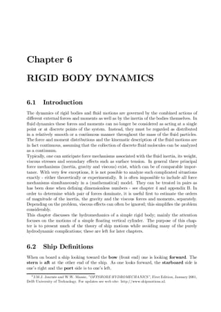
vertical motions of the cylinder are determined by the solid mass m of the cylinder and
the hydromechanical loads on the cylinder.
Applying Newton’s second law for the heaving cylinder:
mÄ
z = sum of all forces on the cylinder
= ¡P + pAw ¡ b_
z ¡ aÄ
z
= ¡P + ½g (T ¡ z) Aw ¡ b_
z ¡ aÄ
z (6.24)
With Archimedes’ law P = ½gT Aw, the linear equation of the heave motion becomes:
j(m + a) Ä
z + b_
z + cz = 0j (6.25)
in which:
z = vertical displacement (m)
P = mg = mass force downwards (N)
m = ½AwT = solid mass of cylinder (kg)
a = hydrodynamic mass coe¢cient (Ns2
/m = kg)
b = hydrodynamic damping coe¢cient (Ns/m = kg/s)
c = ½gAw = restoring spring coe¢cient (N/m = kg/s2
)
Aw = ¼
4
D2 = water plane area (m2)
D = diameter of cylinder (m)
T = draft of cylinder at rest (s)
The terms aÄ
z and b _
z are caused by the hydrodynamic reaction as a result of the movement
of the cylinder with respect to the water. The water is assumed to be ideal and thus to
behave as in a potential ‡ow.
0
5
10
15
20
0 1 2 3 4 5
Vertical Cylinder
D = 1.97 m
T = 4.00 m
Mass + Added Mass
Mass
Frequency (rad/s)
Mass
Coefficients
m,
m+a
(ton)
(a)
0
0.05
0.10
0.15
0.20
0.25
0 1 2 3 4 5
Damping
Frequency (rad/s)
Damping
Coefficient
b
(ton/s)
(b)
Figure 6.8: Mass and Damping of a Heaving Vertical Cylinder

The vertical oscillations of the cylinder will generate waves which propagate radially from
it. Since these waves transport energy, they withdraw energy from the (free) buoy’s oscil-
lations; its motion will die out. This so-called wave damping is proportional to the velocity
of the cylinder _
z in a linear system. The coe¢cient b has the dimension of a mass per
unit of time and is called the (wave or potential) damping coe¢cient. Figure 6.8-b
shows the hydrodynamic damping coe¢cient b of a vertical cylinder as a function of the
frequency of oscillation.
In an actual viscous ‡uid, friction also causes damping, vortices and separation phenomena
quite similar to that discussed in chapter 4. Generally, these viscous contributions to the
damping are non-linear, but they are usually small for most large ‡oating structures; they
are neglected here for now.
The other part of the hydromechanical reaction force aÄ
z is proportional to the vertical
acceleration of the cylinder in a linear system. This force is caused by accelerations that
are given to the water particles near to the cylinder. This part of the force does not dissipate
energy and manifests itself as a standing wave system near the cylinder. The coe¢cient
a has the dimension of a mass and is called the hydrodynamic mass or added mass.
Figure 6.8-a shows the hydrodynamic mass a of a vertical cylinder as a function of the
frequency of oscillation.
In his book, [Newman, 1977] provides added mass coe¢cients for deeply submerged 2-D
and 3-D bodies.
Graphs of the three added mass coe¢cients for 2-D bodies are shown in …gure 6.9. The
added mass m11 corresponds to longitudinal acceleration, m22 to lateral acceleration in
equatorial plane and m66 denotes the rotational added moment of inertia. These poten-
tial coe¢cients have been calculated by using conformal mapping techniques as will be
explained in chapter 7.
Figure 6.9: Added Mass Coe¢cients of 2-D Bodies
Graphs of the three added mass coe¢cients of 3-D spheroids, with a length 2a and a
maximum diameter 2b, are shown in …gure 6.10. In this …gure, the coe¢cients have been

made dimensionless using the mass and moment of inertia of the displaced volume of the
‡uid by the body. The added mass m11 corresponds to longitudinal acceleration, m22 to
lateral acceleration in equatorial plane and m55 denotes the added moment of inertia for
rotation about an axis in the equatorial plane.
Figure 6.10: Added Mass Coe¢cients of Ellipsoids
Note that the potential damping of all these deeply submerged bodies is zero since they
no longer generate waves on the water surface.
Since the bottom of the cylinder used in …gure 6.8 is deep enough under the water surface,
it follows from …gure 6.10 that the added mass a can be approximated by the mass of a
hemisphere of ‡uid with a diameter D. The damping coe¢cient, b, will approach to zero,
because a vertical oscillation of this cylinder will hardly produce waves. The actual ratio
between the added mass and the mass of the hemisphere, as obtained from 3-D calculations,
varies for a cylinder as given in …gure 6.8-a between 0.95 and 1.05.
It appears from experiments that in many cases both the acceleration and the velocity
terms have a su¢ciently linear behavior at small amplitudes; they are linear for practical
purposes. The hydromechanical forces are the total reaction forces of the ‡uid on the
oscillating cylinder, caused by this motion in initially still water:
mÄ
z = Fh with: Fh = ¡aÄ
z ¡ b_
z ¡ cz (6.26)
and the equation of motion for the cylinder with a decaying motion in still water becomes:
(m + a) ¢ Ä
z + b ¢ _
z + c ¢ z = 0 (6.27)
A similar approach can be followed for the other motions. In case of angular motions, for
instance roll motions, the uncoupled equation of motion (now with moment terms) of the
cylinder in still water becomes:

(m + a) ¢ Ä
Á + b ¢ _
Á + c ¢ Á = 0 (6.28)
and the coe¢cients in the acceleration term, a and m, are (added) mass moment of inertia
terms. Coupling between motions will be discussed in chapter 8.
Energy Relations
Suppose the cylinder is carrying out a vertical harmonic oscillation:
z = za sin!t
in initially still water of which the linear equation of motion is given by equation 6.27.
The separate work done by the mass, damping and spring force components in this equation
(force component times distance) per unit of time during one period of oscillation, T , are:
1
T
T
Z
0
f(m + a) ¢ Ä
zg ¢ f _
z ¢ dtg =
¡za
2
(m + a) !3
T
T
Z
0
sin!t ¢ cos !t ¢ dt = 0
1
T
T
Z
0
fb ¢ _
zg ¢ f _
z ¢ dtg =
za
2
b!2
T
T
Z
0
cos2
!t ¢ dt =
1
2
b !2
za
2
1
T
T
Z
0
fc ¢ zg ¢ f _
z ¢ dtg =
za
2
c!
T
T
Z
0
sin!t ¢ cos !t ¢ dt = 0 (6.29)
with:
T = 2¼=! = oscillation period (s)
_
z ¢ dt = dz = distance covered in dt seconds (m)
It is obvious from these equations that only the damping force fb ¢ _
zg dissipates energy;
damping is the reason why the heave motion, z, dies out.
Observe now a ‡oating horizontal cylinder as given in …gure 6.11, carrying out a vertical
harmonic oscillation in initially still water: z = za sin!t, which causes radiated waves
de…ned by: ³ = ³a sin(!t + "). A frequency-dependent relation between the damping
coe¢cient, b, and the amplitude ratio of radiated waves and the vertical oscillation, ³a=za,
can be found; see also [Newman, 1962].
The energy E (the work done per unit of time) provided by the hydrodynamic damping
force is the over one period (T ) integrated damping force (b ¢ _
z) times covered distance
( _
z ¢ dt) divided by the time (T):
E =
1
T
T
Z
0
fb ¢ _
zg ¢ f _
z ¢ dtg
=
1
2
b!2
za
2
(6.30)
This energy provided by the above mentioned hydrodynamic damping force is equal to the
energy dissipated by the radiated waves. This is 2 (radiation of waves to two sides) times

Figure 6.11: Oscillating Horizontal Cylinder
the energy of the waves per unit area (1
2
½g³a
2
) times the covered distance by the radiated
wave energy (cg¢T) in one period (T) times the length of the cylinder (L), divided by the
time (T):
E =
1
T
¢ 2 ¢
½
1
2
½g³a
2
¾
¢ fcg¢T ¢ Lg
=
½g2
³a
2
L
2!
(6.31)
To obtain the right hand side of this equation, use has been made of the de…nition of the
group velocity of the waves in deep water: cg = c=2 = g=(2!); see chapter 5.
Thus, the potential damping coe¢cient per unit of length is de…ned by:
1
2
b !2
za
2
=
½g2
³a
2
L
2!
(6.32)
or: ¯
¯
¯
¯
¯
b
0
=
b
L
=
½g2
!3
µ
³a
za
¶2
¯
¯
¯
¯
¯
(6.33)
Similar approaches can be applied for sway and roll oscillations.
The motions are de…ned here by z = za sin!t. It is obvious that a de…nition of the
body oscillation by z = za cos !t will provide the same results, because this means only
an introduction of a constant phase shift of ¡¼=2 in the body motion as well as in the
generated waves.
Linearisation of Nonlinear damping
In some cases (especially roll motions) viscous e¤ects do in‡uence the damping and can re-
sult in nonlinear damping coe¢cients. Suppose a strongly non-linear roll damping moment,
M, which can be described by:
M = b(1)
¢ _
Á + b(2)
¢
¯
¯
¯ _
Á
¯
¯
¯ ¢ _
Á + b(3)
¢ _
Á
3
(6.34)

The modulus of the roll velocity in the second term is required to give the proper sign to
its contribution. This damping moment can be linearised by stipulating that an identical
amount of energy be dissipated by a linear term with an equivalent linear damping
coe¢cient b(eq)
:
1
T
T
Z
0
n
b(eq)
¢ _
Á
o
¢
n
_
Á ¢ dt
o
=
1
T
T
Z
0
n
b(1)
¢ _
Á + b(2)
¢
¯
¯
¯ _
Á
¯
¯
¯ ¢ _
Á + b(3)
¢ _
Á
3
o
¢
n
_
Á ¢ dt
o
(6.35)
De…ne the roll motion by Á = Áa cos(!t+"Á³), as given in equation 6.9. Then a substitution
of _
Á = ¡Áa! sin(!t + "Á³) in equation 6.35 and the use of some mathematics yields:
¯
¯
¯M = b(eq) ¢ _
Á
¯
¯
¯ with:
¯
¯
¯
¯b(eq) = b(1) +
8
3¼
¢ ! ¢ Áa ¢ b(2) +
3
4
¢ !2 ¢ Á2
a ¢ b(3)
¯
¯
¯
¯ (6.36)
Note that this equivalent linear damping coe¢cient depends on both the frequency and
the amplitude of oscillation.
Restoring Spring Terms
For free ‡oating bodies, restoring ’spring’ terms are present for the heave, roll and pitch
motions only. The restoring spring term for heave has been given already; for the angular
motions they follow from the linearized static stability phenomena as given in chapter 2:
heave : czz = ½gAWL
roll : cÁÁ = ½gO ¢ GM
pitch : cµµ = ½gO ¢ GML
in which GM and GML are the transverse and longitudinal initial metacentric heights.
Free Decay Tests
In case of a pure free heaving cylinder in still water, the linear equation of the heave motion
of the center of gravity, G, of the cylinder is given by equation 6.27:
j(m + a) ¢ Ä
z + b ¢ _
z + c ¢ z = 0j
This equation can be rewritten as:
jÄ
z + 2º ¢ _
z + !0
2 ¢ z = 0j (6.37)
in which the damping coe¢cient and the undamped natural frequency are de…ned by:
¯
¯
¯
¯2º =
b
m + a
¯
¯
¯
¯ (a) and
¯
¯
¯
¯!0
2 =
c
m + a
¯
¯
¯
¯ (b) (6.38)
A non-dimensional damping coe¢cient, ·, is written as:
· =
º
!0
=
b
2
p
(m + a) ¢ c
(6.39)

This damping coe¢cient is written as a fraction between the actual damping coe¢cient,
b, and the critical damping coe¢cient, bcr = 2
p
(m + a) ¢ c; so for critical damping:
·cr = 1. Herewith, the equation of motion 6.37 can be re-written as:
jÄ
z + 2·!0 ¢ _
z + !0
2 ¢ z = 0j (6.40)
The buoy is de‡ected to an initial vertical displacement, za, in still water and then released.
The solution of the equation 6.37 of this decay motion becomes after some mathematics:
z = zae¡ºt
µ
cos !zt +
º
!z
sin!zt
¶
(6.41)
where zae¡ºt
is the decrease of the ”crest” after one period.
Then the logarithmic decrement of the motion is:
ºTz = ·!0Tz = ln
½
z(t)
z(t + Tz)
¾
(6.42)
Because !z
2
= !0
2
¡ º2
for the natural frequency oscillation and the damping is small
(º < 0:20) so that º2
¿ !0
2
, one can neglect º2
here and use !z t !0; this leads to:
!0Tz t !zTz = 2¼ (6.43)
The non-dimensional damping is given now by:
¯
¯
¯
¯· =
1
2¼
ln
½
z(t)
z(t + Tz)
¾¯
¯
¯
¯ = b ¢
!0
2c
(6.44)
These ·-values can easily be found when results of decay tests with a model in still water
are available. These are usually in a form such as is shown in …gure 6.12.
Figure 6.12: Determination of Logarithmic Decrement
Be aware that this damping coe¢cient is determined by assuming an uncoupled heave
motion (no other motions involved). Strictly, this damping coe¢cient is not valid for the
actual coupled motions of a free ‡oating cylinder which will be moving in all directions
simultaneously.

The results of free decay tests are presented by plotting the non-dimensional damping
coe¢cient (obtained from two successive positive or negative maximum displacements zai
and zai+2
by:
¯
¯
¯
¯· =
1
2¼
¢ ln
½
zai
zai+2
¾¯
¯
¯
¯ versus za =
¯
¯
¯
¯
zai
+ zai+2
2
¯
¯
¯
¯ (6.45)
To avoid spreading in the successively determined ·-values, caused by a possible zero-shift
of the measuring signal, double amplitudes can be used instead:
¯
¯
¯
¯· =
1
2¼
¢ ln
½
zai
¡ zai+1
zai+2
¡ zai+3
¾¯
¯
¯
¯ versus za =
¯
¯
¯
¯
zai
¡ zai+1
+ zai+2
¡ zai+3
4
¯
¯
¯
¯ (6.46)
It is obvious that this latter method has preference in case of a record with small amplitudes.
The decay coe¢cient · can therefore be estimated from the decaying oscillation by deter-
mining the ratio between any pair of successive (double) amplitudes. When the damping
is very small and the oscillation decays very slowly, several estimates of the decay can be
obtained from a single record. The method is not really practical when º is much greater
than about 0.2 and is in any case strictly valid for small values of º only. Luckily, this is
generally the case.
The potential mass and damping at the natural frequency can be obtained from all of this.
From equation 6.38-b follows:
¯
¯
¯
¯a =
c
!0
2
¡ m
¯
¯
¯
¯ (6.47)
in which the natural frequency, !0, follows from the measured oscillation period and the
solid mass, m, and the spring coe¢cient, c, are known from the geometry of the body.
From equation 6.38-a, 6.38-b and equation 6.39 follows:
¯
¯
¯
¯b =
2·c
!0
¯
¯
¯
¯ (6.48)
in which · follows from the measured record by using equation 6.45 or 6.46 while c and !0
have to be determined as done for the added mass a.
It is obvious that for a linear system a constant ·-value should be found in relation to
za. Note also that these decay tests provide no information about the relation between
the potential coe¢cients and the frequency of oscillation. Indeed, this is impossible since
decay tests are carried out at one frequency only; the natural frequency.
Forced Oscillation Tests
The relation between the potential coe¢cients and the frequency of oscillation can be found
using forced oscillation tests. A schematic of the experimental set-up for the forced heave
oscillation of a vertical cylinder is given in …gure 6.13. The crank at the top of the …gure
rotates with a constant and chosen frequency, !, causing a vertical motion with amplitude
given by the radial distance from the crank axis to the pin in the slot. Vertical forces are
measured in the rod connecting the exciter to the buoy.
During the forced heave oscillation, the vertical motion of the model is de…ned by:
z(t) = za sin !t (6.49)

Figure 6.13: Forced Oscillation Test
and the heave forces, measured by the transducer, are:
Fz(t) = Fa sin (!t + "Fz) (6.50)
The (linear) equation of motion is given by:
j(m + a) Ä
z + b _
z + cz = Fa sin(!t + "Fz)j (6.51)
The component of the exciting force in phase with the heave motion is associated with
inertia and sti¤ness, while the out-of-phase component is associated with damping.
With:
z = za sin!t
_
z = za! cos !t
Ä
z = ¡za!2
sin!t (6.52)
one obtains:
za
©
¡ (m + a) !2
+ c
ª
sin !t + zab!cos !t = Fa cos "Fz sin !t + Fa sin"Fz cos !t (6.53)
which provides:
from !t =
¼
2
:
¯
¯
¯
¯
¯
a =
c ¡ Fa
za
cos "Fz
!2
¡ m
¯
¯
¯
¯
¯
from !t = 0:
¯
¯
¯
¯
¯
b =
Fa
za
sin "Fz
!
¯
¯
¯
¯
¯
from geometry: jc = ½gAwj (6.54)

To obtain the ’spring’ sti¤ness, c, use has to be made of Aw (area of the waterline), which
can be obtained from the geometry of the model. It is possible to obtain the sti¤ness
coe¢cient from static experiments as well. In such a case equation 6.51 degenerates:
Ä
z = 0 and _
z = 0 yielding: c =
Fz
z
in which z is a constant vertical displacement of the body and Fz is a constant force
(Archimedes’ law).
The in-phase and out-of-phase parts of the exciting force during an oscillation can be found
easily from an integration over a whole number (N ) periods (T) of the measured signal
F(t) multiplied with cos!t and sin !t, respectively:
Fa sin"Fz =
2
N T
NT
Z
0
F(t) ¢ cos !t ¢ dt
Fa cos "Fz =
2
N T
NnT
Z
0
F(t) ¢ sin!t ¢ dt (6.55)
These are nothing more than the …rst order (and averaged) Fourier series components of
F(t); see appendix C:
6.3.3 Wave Loads
Waves are now generated in the test basin for a new series of tests. The object is restrained
so that one now measures (in this vertical cylinder example) the vertical wave load on the
…xed cylinder. This is shown schematically in …gure 6.7-c.
The classic theory of deep water waves (see chapter 5) yields:
wave potential : © =
¡³ag
!
ekz
sin(!t ¡ kx) (6.56)
wave elevation : ³ = ³a cos(!t ¡ kx) (6.57)
so that the pressure, p, on the bottom of the cylinder (z = ¡T) follows from the linearized
Bernoulli equation:
p = ¡½
@©
@t
¡ ½gz
= ½g³aekz
cos(!t ¡ kx) ¡ ½gz
= ½g³ae¡kT
cos(!t ¡ kx) + ½gT (6.58)
Assuming that the diameter of the cylinder is small relative to the wave length (kD t 0),
so that the pressure distribution on the bottom of the cylinder is essentially uniform, then
the pressure becomes:
p = ½g³ae¡kT
cos(!t) + ½gT (6.59)
Then the vertical force on the bottom of the cylinder is:
F =
©
½g³ae¡kT
cos(!t) + ½gT
ª
¢
¼
4
D2
(6.60)

where D is the cylinder diameter and T is the draft.
The harmonic part of this force is the regular harmonic wave force, which will be con-
sidered here. More or less in the same way as with the hydromechanical loads (on the
oscillating body in still water), this wave force can also be expressed as a spring coe¢cient
c times a reduced or e¤ective wave elevation ³¤
:
jFFK = c ¢ ³¤
j with: c = ½g
¼
4
D2
(spring coe¤.)
³¤
= e¡kT
¢ ³a cos(!t) (deep water) (6.61)
This wave force is called the Froude-Krilov force, which follows from an integration of
the pressures on the body in the undisturbed wave.
Actually however, a part of the waves will be di¤racted, requiring a correction of this
Froude-Krilov force. Using the relative motion principle described earlier in this chapter,
one …nds additional force components: one proportional to the vertical acceleration of the
water particles and one proportional to the vertical velocity of the water particles.
The total wave force can be written as:
¯
¯
¯Fw = aÄ
³
¤
+ b_
³
¤
+ c³¤
¯
¯
¯ (6.62)
in which the terms aÄ
³
¤
and b_
³
¤
are considered to be corrections on the Froude-Krilov force
due to di¤raction of the waves by the presence of the cylinder in the ‡uid.
The ”reduced” wave elevation is given by:
³¤
= ³ae¡kT
cos(!t)
_
³
¤
= ¡³ae¡kT
! sin(!t)
Ä
³
¤
= ¡³ae¡kT
!2
cos(!t) (6.63)
A substitution of equations 6.63 in equation 6.62 yields:
Fw = ³ae¡kT
©
c ¡ a!2
ª
cos(!t) ¡ ³ae¡kT
fb!g sin(!t) (6.64)
Also, this wave force can be written independently in terms of in-phase and out-of-phase
terms:
Fw = Fa cos(!t + "F³ )
= Fa cos("F³) cos(!t) ¡ Fa sin("F³ )sin(!t) (6.65)
Equating the two in-phase terms and the two out-of-phase terms in equations 6.64 and
6.65 result in two equations with two unknowns:
Fa cos("F³) = ³ae¡kT
©
c ¡ a!2
ª
Fa sin("F³) = ³ae¡kT
fb!g (6.66)
Adding the squares of these two equations results in the wave force amplitude:
¯
¯
¯
¯
Fa
³a
= e¡kT
q
fc ¡ a!2g
2
+ fb!g
2
¯
¯
¯
¯ (6.67)

and a division of the in-phase and the out-of-phase term in equation 6.66, results in the
phase shift: ¯
¯
¯
¯"F³ = arctan
½
b!
c ¡ a!2
¾
with: 0 · "z³ · 2¼
¯
¯
¯
¯ (6.68)
The phase angle, "F³, has to be determined in the correct quadrant between 0 and 2¼.
This depends on the signs of both the numerator and the denominator in the expression
for the arctangent.
The wave force amplitude, Fa, is proportional to the wave amplitude, ³a, and the phase
shift "F³ is independent of the wave amplitude, ³a; the system is linear.
0
10
20
30
40
0 1 2 3 4 5
without diffraction
with diffraction
Wave Frequency (rad/s)
Wave
Force
Amplitude
F
a
/
ζ
a
(kN/m)
-180
-90
0
0 1 2 3 4 5
without diffraction
with diffraction
Wave Frequency (rad/s)
Wave
Force
Phase
ε
F
ζ
(deg)
Figure 6.14: Vertical Wave Force on a Vertical Cylinder
Figure 6.14 shows the wave force amplitude and phase shift as a function of the wave
frequency. For low frequencies (long waves), the di¤raction part is very small and the wave
force tends to the Froude-Krilov force, c³¤
. At higher frequencies there is an in‡uence of
di¤raction on the wave force on this vertical cylinder. There, the wave force amplitude
remains almost equal to the Froude-Krilov force.
Di¤raction becomes relatively important for this particular cylinder as the Froude-Krylov
force has become small; a phase shift of ¡¼ occurs then quite suddenly. Generally, this
happens the …rst time as the in-phase term, Fa cos("F³), changes sign (goes through zero);
a with ! decreasing positive Froude-Krylov contribution and a with ! increasing negative
di¤raction contribution (hydrodynamic mass times ‡uid acceleration), while the out-of-
phase di¤raction term (hydrodynamic damping times ‡uid velocity), Fa sin("F³), maintains
its sign.
6.3.4 Equation of Motion
Equation 6.23: mÄ
z = Fh + Fw can be written as: mÄ
z ¡ Fh = Fw. Then, the solid mass
term and the hydromechanic loads in the left hand side (given in equation 6.25) and the

exciting wave loads in the right hand side (given in equation 6.62) provides the equation
of motion for this heaving cylinder in waves:
¯
¯
¯(m + a) Ä
z + b _
z + cz = aÄ
³
¤
+ b_
³
¤
+ c³¤
¯
¯
¯ (6.69)
Using the relative motion principle, this equation can also be found directly from Newton’s
second law and the total relative motions of the water particles (Ä
³
¤
, _
³
¤
and ³¤
) of the heaving
cylinder in waves:
mÄ
z = a
³
Ä
³
¤
¡ Ä
z
´
+ b
³
_
³
¤
¡ _
z
´
+ c(³¤
¡ z) (6.70)
In fact, this is also a combination of the equations 6.25 and 6.62.
6.3.5 Response in Regular Waves
The heave response to the regular wave excitation is given by:
z = za cos(!t + "z³ )
_
z = ¡za! sin(!t + "z³ )
Ä
z = ¡za!2
cos(!t + "z³ ) (6.71)
A substitution of 6.71 and 6.63 in the equation of motion 6.69 yields:
za
©
c ¡ (m + a) !2
ª
cos(!t + "z³) ¡ za fb!g sin(!t + "z³ ) =
= ³ae¡kT
©
c ¡ a!2
ª
cos(!t) ¡ ³ae¡kT
fb!gsin(!t) (6.72)
or after splitting the angle (!t + "z³ ) and writing the out-of-phase term and the in-phase
term separately:
za
©©
c ¡ (m + a)!2
ª
cos("z³) ¡ fb!gsin("z³)
ª
cos(!t)
¡za
©©
c ¡ (m + a) !2
ª
sin("z³) + fb!g cos("z³)
ª
sin(!t) =
= ³ae¡kT
©
c ¡ a!2
ª
cos(!t)
¡³ae¡kT
fb!g sin(!t) (6.73)
By equating the two out-of-phase terms and the two in-phase terms, one obtains two
equations with two unknowns:
za
©©
c ¡ (m + a)!2
ª
cos("z³) ¡ fb!gsin("z³)
ª
= ³ae¡kT
©
c ¡ a!2
ª
za
©©
c ¡ (m + a) !2
ª
sin("z³ ) + fb!g cos("z³)
ª
= ³ae¡kT
fb!g (6.74)
Adding the squares of these two equations results in the heave amplitude:
¯
¯
¯
¯
¯
za
³a
= e¡kT
s
fc ¡ a!2g
2
+ fb!g
2
fc ¡ (m + a)!2g
2
+ fb!g
2
¯
¯
¯
¯
¯
(6.75)
and elimination of za=³ae¡kT
in the two equations in 6.74 results in the phase shift:
¯
¯
¯
¯"z³ = arctan
½
¡mb!3
(c ¡ a!2) fc ¡ (m + a) !2g + fb!g
2
¾
with : 0 · "z³ · 2¼
¯
¯
¯
¯ (6.76)

The phase angle "z³ has to be determined in the correct quadrant between 0 and 2¼. This
depends on the signs of both the numerator and the denominator in the expression for the
arctangent.
The requirements of linearity is ful…lled: the heave amplitude za is proportional to the
wave amplitude ³a and the phase shift "z³ is not dependent on the wave amplitude ³a.
Generally, these amplitudes and phase shifts are called:
Fa
³a
(!) and za
³a
(!) = amplitude characteristics
"F³(!) and "z³ (!) = phase characteristics
¾
frequency characteristics
The response amplitude characteristics za
³a
(!) are also referred to as Response Amplitude
Operator (RAO).
0
0.5
1.0
1.5
2.0
0 1 2 3 4 5
without diffraction
with diffraction
Frequency (rad/s)
Heave
amplitude
z
a
/
ζ
a
(-)
-180
-90
0
0 1 2 3 4 5
without diffraction
with diffraction
Frequency (rad/s)
Heave
Phase
ε
z
ζ
(deg)
Figure 6.15: Heave Motions of a Vertical Cylinder
Figure 6.15 shows the frequency characteristics for heave together with the in‡uence of
di¤raction of the waves. The annotation ”without di¤raction” in these …gures means that
the wave load consists of the Froude-Krilov force, c³¤
, only.
Equation 6.75 and …gure 6.16 show that with respect to the motional behavior of this
cylinder three frequency areas can be distinguished:
1. The low frequency area, !2
¿ c=(m + a), with vertical motions dominated by the
restoring spring term.
This yields that the cylinder tends to ”follow” the waves as the frequency decreases;
the RAO tends to 1.0 and the phase lag tends to zero. At very low frequencies, the
wave length is large when compared with the horizontal length (diameter) of the
cylinder and it will ”follow” the waves; the cylinder behaves like a ping-pong ball in
waves.

2. The natural frequency area, !2 t c=(m+a), with vertical motions dominated by the
damping term.
This yields that a high resonance can be expected in case of a small damping. A
phase shift of ¡¼ occurs at about the natural frequency, !2
t c=(m + a); see the
denominator in equation 6.76. This phase shift is very abrupt here, because of the
small damping b of this cylinder.
3. The high frequency area, !2
À c=(m + a), with vertical motions dominated by the
mass term.
This yields that the waves are ”losing” their in‡uence on the behavior of the cylinder;
there are several crests and troughs within the horizontal length (diameter) of the
cylinder. A second phase shift appears at a higher frequency, !2
t c=a; see the
denominator in equation 6.76. This is caused by a phase shift in the wave load.
Figure 6.16: Frequency Areas with Respect to Motional Behavior
Note: From equations 6.67 and 6.75 follow also the heave motion - wave force amplitude
ratio and the phase shift between the heave motion and the wave force:
¯
¯
¯
¯
¯
¯
za
Fa
=
1
q
fc ¡ (m + a)!2g
2
+ fb!g
2
¯
¯
¯
¯
¯
¯
j"zF = "z³ + "³F = "z³ ¡ "F³j (6.77)
6.3.6 Response in Irregular Waves
The wave energy spectrum was de…ned in chapter 5 by:
¯
¯
¯
¯S³ (!) ¢ d! =
1
2
³2
a(!)
¯
¯
¯
¯ (6.78)

Analogous to this, the energy spectrum of the heave response z(!; t) can be de…ned by:
Sz(!) ¢ d! =
1
2
z2
a(!)
=
¯
¯
¯
¯
za
³a
(!)
¯
¯
¯
¯
2
¢
1
2
³2
a(!)
=
¯
¯
¯
¯
za
³a
(!)
¯
¯
¯
¯
2
¢ S³(!) ¢ d! (6.79)
Thus, the heave response spectrum of a motion can be found by using the transfer func-
tion of the motion and the wave spectrum by:
¯
¯
¯
¯
¯
Sz(!) =
¯
¯
¯
¯
za
³a
(!)
¯
¯
¯
¯
2
¢ S³(!)
¯
¯
¯
¯
¯
(6.80)
The principle of this transformation of wave energy to response energy is shown in …gure
6.17 for the heave motions being considered here.
The irregular wave history, ³(t) - below in the left hand side of the …gure - is the sum of
a large number of regular wave components, each with its own frequency, amplitude and
a random phase shift. The value 1
2
³2
a(!)=¢! - associated with each wave component on
the !-axis - is plotted vertically on the left; this is the wave energy spectrum, S³(!). This
part of the …gure can be found in chapter 5 as well, by the way.
Each regular wave component can be transferred to a regular heave component by a mul-
tiplication with the transfer function za=³a(!). The result is given in the right hand side
of this …gure. The irregular heave history, z(t), is obtained by adding up the regular heave
components, just as was done for the waves on the left. Plotting the value 1
2z2
a(!)=¢!
of each heave component on the !-axis on the right yields the heave response spectrum,
Sz(!).
The moments of the heave response spectrum are given by:
¯
¯
¯
¯
¯
¯
mnz =
1
Z
0
Sz(!) ¢ !n ¢ d!
¯
¯
¯
¯
¯
¯
with: n = 0; 1; 2; ::: (6.81)
where n = 0 provides the area, n = 1 the …rst moment and n = 2 the moment of inertia of
the spectral curve.
The signi…cant heave amplitude can be calculated from the spectral density function of the
heave motions, just as was done for waves. This signi…cant heave amplitude, de…ned
as the mean value of the highest one-third part of the amplitudes, is:
¯
¯
¯¹
za1=3
= 2 ¢ RMS = 2
p
m0z
¯
¯
¯ (6.82)
in which RMS (=
p
m0z) is the Root Mean Square value.
A mean period can be found from the centroid of the spectrum:
¯
¯
¯
¯T1z = 2¼ ¢
m0z
m1z
¯
¯
¯
¯ (6.83)

Figure 6.17: Principle of Transfer of Waves into Responses
Another de…nition, which is equivalent to the average zero-crossing period, is found
from the spectral radius of gyration:
¯
¯
¯
¯T2z = 2¼ ¢
r
m0z
m2z
¯
¯
¯
¯ (6.84)
6.3.7 Spectrum Axis Transformation
When wave spectra are given as a function of frequencies in Herz (f = 1=T ) and one needs
this on an !-basis (in radians/sec), they have to be transformed just as was done for waves
in chapter 5. The heave spectrum on this !-basis becomes:
Sz(!) =
Sz(f)
2¼
=
¯
¯
¯
¯
za
³a
(f or !)
¯
¯
¯
¯
2
¢
S³(f)
2¼
(6.85)

6.4. SECOND ORDER WAVE DRIFT FORCES 6-27
6.4 Second Order Wave Drift Forces
Now that the …rst order behavior of linear (both mechanical as well as hydromechanical)
systems has been handled, attention in the rest of this chapter shifts to nonlinear systems.
Obviously hydrodynamics will get the most emphasis in this section, too.
The e¤ects of second order wave forces are most apparent in the behavior of anchored
or moored ‡oating structures. In contrast to what has been handled above, these are
horizontally restrained by some form of mooring system. Analyses of the horizontal motions
of moored or anchored ‡oating structures in a seaway show that the responses of the
structure on the irregular waves include three important components:
1. A mean displacement of the structure, resulting from a constant load component.
Obvious sources of these loads are current and wind. In addition to these, there is
also a so-called mean wave drift force. This drift force is caused by non-linear
(second order) wave potential e¤ects. Together with the mooring system, these loads
determine the new equilibrium position - possibly both a translation and (in‡uenced
by the mooring system) a yaw angle - of the structure in the earth-bound coordinate
system. This yaw is of importance for the determination of the wave attack angle.
2. An oscillating displacement of the structure at frequencies corresponding to those of
the waves; the wave-frequency region.
These are linear motions with a harmonic character, caused by the …rst order wave
loads. The principle of this has been presented above for the vertically oscillating
cylinder. The time-averaged value of this wave load and the resulting motion com-
ponent are zero.
3. An oscillating displacement of the structure at frequencies which are much lower than
those of the irregular waves; the low-frequency region.
These motions are caused by non-linear elements in the wave loads, the low-frequency
wave drift forces, in combination with spring characteristics of the mooring system.
Generally, a moored ship has a low natural frequency in its horizontal modes of mo-
tion as well as very little damping at such frequencies. Very large motion amplitudes
can then result at resonance so that a major part of the ship’s dynamic displacement
(and resulting loads in the mooring system) can be caused by these low-frequency
excitations.
Item 2 of this list has been discussed in earlier parts of this chapter; the discussion of item
1 starts below; item 3 is picked up later in this chapter and along with item 1 again in
chapter 9.
6.4.1 Mean Wave Loads on a Wall
Mean wave loads in regular waves on a wall can be calculated simply from the pressure in the
‡uid, now using the more complete (not-linearized!) Bernoulli equation. The superposition
principle can still be used to determine these loads in irregular waves. When the waves are
not too long, this procedure can be used, too, to estimate the mean wave drift forces on a
ship in beam waves (waves approaching from the side of the ship).

Regular Waves
A regular wave (in deep water) hits a vertical wall with an in…nite depth as shown in …gure
6.18. This wave will be re‡ected fully, so that a standing wave (as described in chapter 5)
results at the wall.
Figure 6.18: Regular Wave at a Wall
The incident undisturbed wave is de…ned by:
¯
¯
¯
¯©i = ¡
³ag
!
¢ ekz ¢ sin(+kx + !t)
¯
¯
¯
¯ and j³i = ³a ¢ cos(+kx + !t)j (6.86)
and the re‡ected wave by:
¯
¯
¯
¯©r = ¡
³ag
!
¢ ekz ¢ sin(¡kx + !t)
¯
¯
¯
¯ and j³r = ³a ¢ cos(¡kx + !t)j (6.87)
Then the total wave system can be determined by a superposition of these two waves; this
results in a standing wave system:
© = ©i + ©r = ¡2 ¢
³ag
!
¢ ekz
¢ cos(kx) ¢ sin(!t)
³ = ³i + ³r = 2 ¢ ³a ¢ cos(kx) ¢ cos(!t) (6.88)
The pressure in the ‡uid follows from the complete Bernoulli equation:
p = ¡½g ¢ z ¡ ½ ¢
@©
@t
¡
1
2
½ ¢ (r©)
2
= ¡½g ¢ z ¡ ½ ¢
@©
@t
¡
1
2
½ ¢
(µ
@©
@x
¶2
+
µ
@©
@z
¶2
)
(6.89)
The derivatives of the potential ©(x; z; t) with respect to t, x and z are given by:
@©
@t
= ¡2 ¢ ³a ¢ g ¢ ekz
¢ cos(kx) ¢ cos(!t)
u =
@©
@x
= +2 ¢ ³a ¢ ! ¢ ekz
¢ sin(kx) ¢ sin(!t)
w =
@©
@z
= ¡2 ¢ ³a ¢ ! ¢ ekz
¢ cos(kx) ¢ sin(!t) (6.90)

At the wall (x = 0), the wave elevation and the derivatives of the potential are:
³ = 2 ¢ ³a ¢ cos(!t)
@©
@t
= ¡2 ¢ ³a ¢ g ¢ ekz
¢ cos(!t)
u =
@©
@x
= 0
w =
@©
@z
= ¡2 ¢ ³a ¢ ! ¢ ekz
¢ sin(!t) (6.91)
and the pressure on the wall is:
p = ¡½g ¢ z ¡ ½ ¢
@©
@t
¡
1
2
½ ¢
(µ
@©
@x
¶2
+
µ
@©
@z
¶2
)
= ¡½g ¢ z + 2½g ¢ ³a ¢ ekz
¢ cos(!t) ¡
1
2
½ ¢
¡
4³a
2
¢ !2
¢ e2kz
sin2
(!t)
¢
= ¡½g ¢ z + 2½g ¢ ³a ¢ ekz
¢ cos(!t) ¡ ½ ¢ ³a
2
¢ !2
¢ e2kz
¢ (1 ¡ cos(2!t)) (6.92)
This time-varying pressure on the wall can also be written as:
p = ¹
p(0)
+ ~
p(1)
+ ¹
p(2)
+ ~
p(2)
(6.93)
where:
¹
p(0)
= ¡½g ¢ z
~
p(1)
= +2½g ¢ ³a ¢ ekz
¢ cos(!t)
¹
p(2)
= ¡½ ¢ ³a
2
¢ !2
¢ e2kz
~
p(2)
= +½ ¢ ³a
2
¢ !2
¢ e2kz
¢ cos(2!t) (6.94)
The general expression for the mean force on the wall follows from:
F = ¡
³
Z
¡1
(¹
p ¢ ¹
n) ¢ dS (6.95)
where the superscript bar over the entire integral indicates a (long) time average.
Because ¹
n = (1; 0; 0) and dS = 1 ¢ dz, this mean force becomes:
¹
F = ¡
³(t)
Z
¡1
p(z; t) ¢ dz (6.96)
which is split into two parts over the vertical axis; one above and one below the still water
level:
¹
F = ¡
0
Z
¡1
p(z; t) ¢ dz ¡
³(t)
Z
0
p(z; t) ¢ dz (6.97)
= F1 + F2 (6.98)

where:
p(z; t) = ¹
p(0)
+ ~
p(1)
+ ¹
p(2)
+ ~
p(2)
and ³(t) = ~
³
(1)
(t) (6.99)
The …rst part F1 comes from the integration from ¡1 to 0; it contributes to the integration
of ¹
p(0) and ¹
p(2) only:
F1 = ¡
0
Z
¡1
p(z; t) ¢ dz
= ¡
0
Z
¡1
¡
¡½gz ¡ ½ ¢ ³a
2
¢ !2
¢ e2kz
¢
¢ dz
= ½ ¢ !2
¢ ³a
2
0
Z
¡1
e2kz
¢ dz
= +
1
2
½g ¢ ³a
2
(6.100)
This force is directed away from the wall. The static …rst term (¡½gz) has been left out
of consideration, while the dispersion relation for deep water (!2
= kg) has been utilized
in the second term.
The second part, F2, comes from the integration from 0 to ³(t); it contributes to the
integration of ¹
p(0)
and ~
p(1)
only, so that the time-dependent force F2(t) becomes:
F2(t) = ¡
³(t)
Z
0
p(z; t) ¢ dz
= ¡
³(t)
Z
0
(¡½g ¢ z + ½g ¢ ³(t)) ¢ dz
= +½g
³(t)
Z
0
z ¢ dz ¡ ½g
³(t)
Z
0
³(t) ¢ dz
= +
1
2
½g ¢ f³(t)g2
¡ ½g ¢ f³(t)g2
= ¡
1
2
½g ¢ f³(t)g2
(6.101)
Because
³(t) = 2 ¢ ³a ¢ cos(!t) and cos2
(!t) =
1
2
¢ (1 + cos(2!t)) (6.102)
this part of the force becomes:
F2(t) = ¡
1
2
½g ¢ 4 ¢ ³a
2
¢ cos2
(!t)
= ¡½g ¢ ³a
2
¢ (1 + cos(2!t)) (6.103)

Figure 6.19: Mean Wave Loads on a Wall
The desired time-averaged value becomes:
F2 = ¡½g ¢ ³a
2
(6.104)
where ³a is the amplitude of the incoming wave. This force is directed toward the wall.
Finally, see …gure 6.19, the total time-averaged force ¹
F per meter length of the wall be-
comes:
¹
F = F1 + F2
= +
1
2
½g ¢ ³a
2
¡ ½g ¢ ³a
2
(6.105)
Thus: ¯
¯
¯
¯
¹
F = ¡
1
2
½g ¢ ³a
2
¯
¯
¯
¯ (6.106)
in which it is assumed that the incident wave is fully re‡ected. This total force has a
magnitude proportional to the square of the incoming wave amplitude and it is directed
toward the wall.
Note that this force is also directly related to the energy per unit area of the incoming
waves as found in chapter 5:
E =
1
2
½g ¢ ³2
a (6.107)
Comparison of equations 6.106 and 6.107 reveals that the mean wave drift force is numer-
ically equal to the energy per unit area of the incoming waves.
Irregular Waves
The discovery just made above will be utilized to determine the mean wave drift force from
irregular waves as well. This is done via the wave spectrum, de…ned by:
S³(!) ¢ d! =
1
2
³a
2
(!) with a zero order moment: m0 =
1
Z
0
S³ (!) ¢ d! (6.108)
Then the total force on the wall can be written as:
¹
F = ¡
X 1
2
½g ¢ ³a
2
(!)

= ¡½g
1
Z
0
S³(!) ¢ d!
= ¡½g ¢ m0³ (6.109)
Because:
H1=3 = 4
p
m0³ or m0³ =
1
16
¢ H1=3
2
(6.110)
it follows that the mean wave drift force can be expressed as:
¯
¯
¯
¯
¹
F =
¡1
16
¢ ½g ¢ H1=3
2
¯
¯
¯
¯ per metre length of the wall (6.111)
Approximation for Ships
It has been assumed so far that the incident wave is fully re‡ected. When the waves are not
too long, so that the water motion is more or less concentrated near the sea surface (over
the draft of the ship), full re‡ection can be assumed for large ships too. Then, equation
6.111 can be used for a …rst estimation of the mean wave drift forces on a ship in beam
waves.
The mean wave drift force on an example ship with a length L of 300 meters in beam waves
with a signi…cant wave height H1=3 of 4.0 meters can be approximated easily. Assuming
that all waves will be re‡ected, the mean wave drift force is:
¹
F =
1
16
¢ ½g ¢ H1=3
2
¢ L
=
1
16
¢ 1:025 ¢ 9:806 ¢ 4:02
¢ 300 ¼ 3000 kN (6.112)
6.4.2 Mean Wave Drift Forces
[Maruo, 1960] showed for the two-dimensional case of an in…nitely long cylinder ‡oating in
regular waves with its axis perpendicular to the wave direction that the mean wave drift
force per unit length satis…es: ¯
¯
¯
¯
¹
F 0
=
1
2
½g ¢ ³ar
2
¯
¯
¯
¯ (6.113)
in which ³ar is the amplitude of the wave re‡ected and scattered by the body in a direction
opposite to the incident wave.
Generally only a part of the incident regular wave will be re‡ected; the rest will be trans-
mitted underneath the ‡oating body. Besides the re‡ected wave, additional waves are
generated by the heave, pitch and roll motions of the vessel. The re‡ected and scattered
waves have the same frequency as the incoming wave, so that the sum of these compo-
nents still has the same frequency as the incoming wave. Their amplitudes will depend on
the amplitudes and relative phases of the re‡ected and scattered wave components. The
amplitudes of these components and their phase di¤erences depend on the frequency of
the incident wave, while the amplitudes can be assumed to be linearly proportional to the
amplitude of the incident wave. This is because it is the incident wave amplitude which
causes the body to move in the …rst place. In equation form:
³ar = R(!) ¢ ³a (6.114)

in which R(!) is a re‡ection coe¢cient.
This means that the mean wave drift force in regular waves per meter length of the cylinder
can be written as:
¯
¯
¯
¯F
0
d =
1
2
½g ¢ fR(!) ¢ ³ag
2
¯
¯
¯
¯ (6.115)
This expression indicates that the mean wave drift force is proportional to the incident
wave amplitude squared. Note that in case of the previously discussed wall: R(!) = 1:0.
6.4.3 Low-Frequency Wave Drift Forces
[Hsu and Blenkarn, 1970] and [Remery and Hermans, 1971] studied the phenomenon of the
mean and slowly varying wave drift forces in a random sea from the results of model tests
with a rectangular barge with breadth B. It was moored in irregular head waves to a
…xed point by means of a bow hawser. The wave amplitudes provide information about
the slowly varying wave envelope of an irregular wave train. The wave envelope is an
imaginary curve joining successive wave crests (or troughs); the entire water surface motion
takes place with the area enclosed by these two curves.
It seems logical in the light of the earlier results to expect that the square of the envelope
amplitude will provide information about the drift forces in irregular waves. To do this,
one would (in principle) make a spectral analysis of the square of this wave envelope. In
other words, the spectral density of the square of the wave amplitude provides information
about the mean period and the magnitude of the slowly varying wave drift force.
In practice it is very di¢cult to obtain an accurate wave envelope spectrum due to the
long wave record required. Assuming that about 200-250 oscillations are required for an
accurate spectral analysis and that the mean period of the wave envelope record is about
100 seconds, the total time that the wave elevation has to be recorded can be up to 7 hours.
Another very simple method is based on individual waves in an irregular wave train. As-
sume that the irregular wave train is made up of a sequence of single waves of which the
wave amplitude is characterized by the height of a wave crest or the depth of a wave trough,
³ai, while the period, Ti, (or really half its value) is determined by the two adjacent zero
crossings (see …gure 6.20).
Figure 6.20: Wave Drift Forces Obtained from a Wave Record

Each of the so obtained single waves (one for every crest or trough) is considered to be one
out of a regular wave train, which exerts (in this case) a surge drift force on the barge:
Fi =
1
2
½g ¢ fR(!i) ¢ ³aig
2
¢ B with: !i =
2¼
Ti
(6.116)
When this is done for all wave crests and troughs in a wave train, points on a curve
representing a slowly varying wave drift force, F(t), will be obtained. This drift force
consists of a slowly varying force (the low-frequency wave drift force) around a mean value
(the mean wave drift force); see …gure 6.20.
Figure 6.21: Low-Frequency Surge Motions of a Barge
These low-frequency wave drift forces on the barge will induce low-frequency surge motions
with periods of for instance over 100 seconds. An example is given in …gure 6.21 for two
di¤erent spring constants, C. The period ratio, ¤, in this …gure is the ratio between the
natural surge period of the system (ship plus mooring) and the wave envelope period.
(Another term for the wave envelope period is wave group period.) As can be seen
in this …gure the …rst order (wave-frequency) surge motions are relatively small, when
compared with the second order (low-frequency) motions. This becomes especially true
near resonance (when ¤ ! 1:0).
Resonance may occur when wave groups are present with a period in the vicinity of the
natural period of the mooring system. Due to the low natural frequency for surge of the
bow hawser - barge system and the low damping at this frequency, large surge motions can

result. According to [Remery and Hermans, 1971], severe horizontal motions can be built
up within a time duration of only a few consecutive wave groups. Obviously, information
about the occurrence of wave groups will be needed to predict this response. This is a
matter for oceanographers.
6.4.4 Additional Responses
The table below summarizes possible responses of a system (such as a moored vessel) to
regular and irregular waves. Both linear and nonlinear mooring systems are included here;
mooring systems can be designed to have nearly linear characteristics, but most are at
least a bit nonlinear.
The right hand side of the table below gives the motions which are possible via each of the
’paths’ from left to right. There will always be …rst order response to …rst order excitations;
these have been discussed already as has the response of a linear or non-linear system to
higher order excitations.
Wave Excitation System Response
Regular First order Linear
First order
(single frequency)
Regular First order Nonlinear
Subharmonic
(single low frequency)
Regular Higher order Linear
Time-independent
drift
Regular Higher order Nonlinear
Time-independent
drift
Irregular First order Linear
First order
(wave frequencies)
Irregular First order Nonlinear
Subharmonic
(uncertain)
Irregular Higher order Linear
Time-dependent
drift
Irregular Higher order Nonlinear
Time-dependent
drift
Subharmonic Response
One path in the table above has not been discussed yet. This involves a subharmonic
response of a nonlinear system to a …rst order excitation from either regular or irregular
waves. The response, itself, looks much like the response to slow drift forces; these two are
di¢cult indeed to distinguish. Luckily perhaps, a signi…cant time is needed to build up

subharmonic resonant motions of high amplitude. This implies that the excitation must
remain very nicely behaved over quite some time in order for this to happen. Waves at sea
are very often too irregular; this subharmonic motion breaks down before large amplitudes
are generated.
6.5 Time Domain Approach
If (as has been assumed so far in most of this chapter) the system is linear, such that its
behavior is linearly related to its displacement, velocity and acceleration, then the behavior
of the system can be studied in the frequency domain.
However, in a lot of cases there are several complications which violate this linear assump-
tion, for instance nonlinear viscous damping, forces and moments due to currents, wind,
anchoring and not to mention second order wave loads. If the system is nonlinear, then
superposition principle - the foundation of the frequency domain approach - is no longer
valid. Instead, one is forced to revert to the direct solution of the equations of motion as
functions of time. These equations of motion result directly from Newton’s second law.
Approaches to their solution are presented in this section.
6.5.1 Impulse Response Functions
The hydromechanical reaction forces and moments, due to time varying ship motions,
can be described using the classic formulation given by [Cummins, 1962]. Complex po-
tential problems, can be handled via frequency-dependent potential coe¢cients as done by
[Ogilvie, 1964]. The principle of this approach will be demonstrated here for a motion with
one degree of freedom. Insight about the possibilities of this method is more important in
this section than the details of the derivations involved; the result is more important than
the exact route leading to it.
Cummins Equation
The ‡oating object is assumed to be a linear system with a translational (or rotational)
velocity as input and the reaction force (or moment) of the surrounding water as output.
The object is assumed to be at rest at time t = t0.
During a short time interval, ¢t, the body experiences an impulsive displacement, ¢x,
with a constant velocity, V , so that:
¢x = V ¢ ¢t (6.117)
During this impulsive displacement, the water particles will start to move. Since potential
‡ow is assumed, a velocity potential, ©, proportional to the velocity, V , can be de…ned:
©(x; y; z; t) = ª(x; y; z) ¢ V (t) for: t0 < t < t0 + ¢t (6.118)
in which ª is the normalized velocity potential.
Note: This ª is not a stream function as used in chapter 3; this notation is used here to
remain consistent with other literature.

6.5. TIME DOMAIN APPROACH 6-37
The water particles are still moving after this impulsive displacement, ¢x. Because the
system is assumed to be linear, the motions of the ‡uid, described by the velocity potential,
©, are proportional to the impulsive displacement, ¢x. So:
©(x; y; z; t) = Â(x; y; z; t) ¢ ¢x for: t > t0 + ¢t (6.119)
in which Â is another normalized velocity potential.
A general conclusion can be that the impulsive displacement, ¢x, during the time interval
(t0; t0 + ¢t) in‡uences the motions of the ‡uid during this interval as well as during all
later time intervals. Similarly, the motions during the interval (t0; t0 + ¢t) are in‡uenced
by the motions before this interval; the system has a form of ”memory”.
When the object performs an arbitrarily time-dependent varying motion, this motion can
be considered to be a succession of small impulsive displacements, so that then the resulting
total velocity potential, ©(t), during the interval (tm; tm + ¢t) becomes:
©(t) = Vm ¢ ª +
m
X
k=1
fÂ(tm¡k; tm¡k + ¢t) ¢ Vk ¢ ¢tg (6.120)
with:
m = number of time steps (-)
tm = t0 + m ¢ ¢t (s)
tm¡k = t0 + (m ¡ k) ¢ ¢t (s)
Vm = velocity component during time interval (tm; tm + ¢t) (m/s)
Vk = velocity component during time interval (tm¡k; tm¡k + ¢t) (m/s)
ª = normalized velocity potential caused by a displacement
during time interval (tm; tm + ¢t)
Â = normalized velocity potential caused by a displacement
during time interval (tm¡k; tm¡k + ¢t)
Letting ¢t go to zero, yields:
©(t) = _
x(t) ¢ ª +
t
Z
¡1
Â(t ¡ ¿) ¢ _
x(¿) ¢ d¿ (6.121)
in which _
x(¿) is the velocity component of the body at time ¿.
The pressure in the ‡uid follows from the linearized Bernoulli equation:
p = ¡½ ¢
@©
@t
(6.122)
An integration of these pressures over the wetted surface, S, of the ‡oating object yields
the expression for the hydrodynamic reaction force (or moment), F .
With n is the generalized directional cosine in a vector notation, F becomes:
F = ¡
Z Z
S
p ¢ n ¢ dS
=
8
<
:
½
Z Z
S
ª ¢ n ¢ dS
9
=
;
¢ Ä
x(t)
+
t
Z
¡1
8
<
:
½
Z Z
S
@Â(t ¡ ¿)
@t
¢ n ¢ dS
9
=
;
¢ _
x(¿) ¢ d¿ (6.123)

By de…ning:
A = ½
Z Z
S
ª ¢ n ¢ dS
B(t) = ½
Z Z
S
@Â(t ¡ ¿)
@t
¢ n ¢ dS (6.124)
the hydrodynamic force (or moment) becomes:
F = A ¢ Ä
x(t) +
t
Z
¡1
B(t ¡ ¿) ¢ _
x(¿) ¢ d¿ (6.125)
Together with a linear restoring spring term C¢x and a linear external load, X(t), Newton’s
second law yields the linear equation of motion in the time domain:
(M + A) ¢ Ä
x(t) +
t
Z
¡1
B(t ¡ ¿) ¢ _
x(¿) ¢ d¿ + C ¢ x(t) = X(t) (6.126)
in which:
Ä
x(t) = translational (or rotational) acceleration at time t (m/s2
)
_
x(t) = translational (or rotational) velocity in at time t (m/s)
x(t) = translational (or rotational) displacement at time t (m)
M = solid mass or mass moment of inertia (kg)
A = hydrodynamic (or added) mass coe¢cient (kg)
B(t), B(¿) = retardation functions (Ns/m)
C = spring coe¢cient from ship geometry (N/m)
X(t) = external load in at time t (N)
t, ¿ = time (s)
By replacing ”¿” by ”t¡ ¿” in the damping part and changing the integration boundaries,
this part can be written in a more convenient form:
¯
¯
¯
¯
¯
¯
(M + A) ¢ Ä
x(t) +
1
Z
0
B(¿) ¢ _
x(t ¡ ¿) ¢ d¿ + C ¢ x(t) = X(t)
¯
¯
¯
¯
¯
¯
(6.127)
This type of equation is often referred to as a ”Cummins Equation” in honor of his work;
see [Cummins, 1962].
Coe¢cient Determination
If present, the linear restoring (hydrostatic) spring coe¢cient, C; can be determined easily
from the underwater geometry and - when rotations are involved - the center of gravity of
the ‡oating object.
The velocity potentials, ª and Â, have to be found to determine the coe¢cients, A and
B. A direct approach is rather complex. An easier method to determine A and B has

been found by [Ogilvie, 1964]. He made use of the hydrodynamic mass and damping data
determined using existing frequency domain computer programs based on potential theory.
This allowed him to express the needed coe¢cients A and B relatively simply in terms of
the calculated hydrodynamic mass and damping data. His approach is developed here.
The ‡oating object is assumed to carry out an harmonic oscillation with a unit amplitude:
x = 1:0 ¢ cos(!t) (6.128)
Substitution of this in the Cummins equation 6.127 yields:
¡!2
¢ (M + A) ¢ cos(!t) ¡ ! ¢
1
Z
0
B(¿) ¢ sin(!t ¡ !¿) ¢ d¿ + C ¢ cos(!t) = X(t) (6.129)
which can be worked out to yield:
¡!2
¢
8
<
:
M + A ¡
1
!
¢
1
Z
0
B(¿)sin(!¿)d¿
9
=
;
¢ cos(!t)
¡!¢
8
<
:
1
Z
0
B(¿) ¢ cos(!¿) ¢ d¿
9
=
;
sin(!t) + fCg ¢ cos(!t) = X(t) (6.130)
Alternatively, the classical frequency domain description of this motion is given by:
¡!2
¢ fM + a(!)g ¢ cos(!t)
¡!¢ fb(!)g ¢ sin(!t) + fcg ¢ cos(!t) = X(t) (6.131)
with:
a(!) = frequency-dependent hydrodynamic mass coe¢cient (Ns2
/m = kg)
b(!) = frequency-dependent hydrodynamic damping coe¢cient (Ns/m)
c = restoring spring term coe¢cient (N/m)
X(t) = external force (N)
[Ogilvie, 1964] compared the time domain and frequency domain equations 6.130 and 6.131
and found:
a(!) = A ¡
1
!
¢
1
Z
0
B(¿) sin(!¿)d¿
b(!) =
1
Z
0
B(¿) ¢ cos(!¿) ¢ d¿
c = C (6.132)
The …rst two of these equations look very similar to those for determining the …rst order
coe¢cients in a Fourier series; see appendix C. An inverse Fourier Transform can be used
to isolate the desired function, B(¿); the coe¢cient, A, can be evaluated directly with a
bit of algebra.

This yields the so-called retardation function:
¯
¯
¯
¯
¯
¯
B(¿) =
2
¼
¢
1
Z
0
b(!) ¢ cos(!¿) ¢ d!
¯
¯
¯
¯
¯
¯
(6.133)
The mass term is simply:
A = a(!) +
1
!
¢
1
Z
0
B(¿) ¢ sin(!¿) ¢ d¿ (6.134)
This expression is valid for any value of !, and thus also for ! = 1; this provides:
jA = a (!) evaluated at ! = 1j (6.135)
The numerical computational problems that have to be solved, because the integrations
have to be carried out from 0 to 1, are not discussed here.
Figure 6.22, is an example of the retardation function for roll of a ship.
Figure 6.22: Retardation Function for Roll
Addition of (External) Loads
So far, discussion has concentrated on the left hand side of equation 6.127. Notice that
this part of the equation is still linear!
Attention shifts now to the right hand side, the external force X(t). Since it can be
convenient to keep the left hand side of the equation of motion linear, one often moves
all the nonlinear e¤ects - even a nonlinear damping or spring force - to the opposite side,
where they are all considered to be part of the external force X(t).
Obviously one will have to know (or at least be able to evaluate) X(t) in order to obtain
a solution to the equation of motion.
Since the …rst order wave force is a linear phenomenon, time histories of the …rst order
wave loads in a certain sea state can be obtained from frequency domain calculations by
using the frequency characteristics of the …rst order wave loads and the wave spectrum by
using the superposition principle:
³(t) =
N
X
n=1
³an
cos(!nt + "n)

with randomly chosen phase shifts, "n, between 0 and 2¼ and:
³an
=
q
2 ¢ S³(!n) ¢ ¢! which follows from:
1
2
³2
an
= S³(!n) ¢ ¢!
see chapter 5.
With this, the time history of the …rst order wave load then becomes:
¯
¯
¯
¯
¯
Xw(t) =
N
X
n=1
µ
Xwan
³an
¶
¢ ³an
cos(!nt + "n + "Xw³n
)
¯
¯
¯
¯
¯
(6.136)
in which:
Xw(t) = wave load (N)
N = number of frequencies (-)
!n = wave frequency rad/s)
Xwan
³an
= transfer function of wave load (N/m)
"Xw³n
= phase shift of wave load (rad)
"n = phase shift of wave (rad)
Note that with a constant frequency interval , ¢!, this time history repeats itself after
2¼=¢! seconds.
With known coe¢cients and the right hand side of this equation of motion, equation 6.127
can be integrated a numerically. Comparisons of calculated and transformed linear motions
in the frequency domain with time domain results show a perfect agreement.
Validation Tests
A series of simple model experiments have been carried out to validate the time domain
calculation routines with non-linear terms. Towing tank number 2 of the Delft Ship Hydro-
mechanics Laboratory with a 1:40 model of the Oil Skimming Vessel m.v. Smal Agt (51.00
x 9.05 x 3.25 meter) was used for this. Horizontal impulse forces in the longitudinal and
lateral direction have been introduced in a tow line between a torque-motor and the model
in still water. The measured motions of the ship model have been compared with the data
calculated in the time domain, using the measured time-series of the impulse forces and
assumed points of application as an input. An example of the comparison is presented in
…gure 6.23 for the sway velocities due to a lateral impulse force amidships.
The …gure shows a good agreement between the calculated and the measured sway motions.
Comparable agreements have been found for the other tests.
A few years ago, the Centre for Applied Research in The Netherlands (TNO) carried out a
series of full scale collision tests with two inland waterway tankers in still water, see …gure
6.24. The contact forces between the two ships and the motions of the rammed ship (80.00
x 8.15 x 2.20 meter) were measured. Computer simulations of the motion behavior of the
rammed ship during the collision have been carried out, using the measured contact forces
on the rammed ship as an input.
Figure 6.25 shows some comparative results for a test with a collision of the rammed ship
at about 0.40 Lpp from the bow on the port side. The ramming ship had a speed of about
15 km/hr. The measured and calculated motions of the rammed ship are presented. Sway,
roll and yaw velocities are predicted here very well.

Figure 6.23: External Impulse and Resulting Motions
Figure 6.24: Underwater Portion of Rammed Ship
6.5.2 Direct Time Domain Simulation
Retardation functions as described above can be used to solve the equations of motion
for cases in which the nonlinearities can be included in the time-dependent excitation on
the right hand side of the equation. While it is possible to ”move” some nonlinearities to
the excitation side of the equation of motion more or less arti…cially, there are still many
relevant physical systems which do not lend themselves to such a treatment.
One example of such a system will come up at the end of chapter 12 when the hydrodynamic
drag on a moving cylinder in waves will be discussed. A perhaps more spectacular example
involves the launching of an o¤shore tower structure from a barge. It should be obvious
that the hydrodynamic mass and damping of such a structure - and of the barge from
which it is launched - will change quite rapidly as the tower enters the water and load is
transferred from the barge. Notice, now, that the hydromechanical coe¢cients - for both
the tower and barge - can best be expressed as (nonlinear) functions of the position of the
respective structures rather than of time. These functions can easily be accommodated in
a time domain calculation in which all conditions can be re-evaluated at the start of each
time step.

Figure 6.25: Measured and Calculated Velocities During a Ship Collision
Indeed, any system can be solved by direct integration of the equations of motion in the
time domain. This approach is direct and certainly straightforward in theory, but it is
often so cumbersome to carry out that it becomes impractical in practice. Admittedly,
modern computers continue to shift the limits of practicality, but these limits are still very
present for many o¤shore engineering applications.
Basic Approach
The approach is simple enough: the di¤erential equations of motion resulting from the
application of Newton’s law are simply integrated - using an appropriate numerical method
- in the time domain. This means that all of the input (such as a wave record) must be
known as a function of time, and that a time record of the output (such as a time history
of hydrodynamic force on a vibrating cable) will be generated.
Di¢culties
A …rst and obvious di¢culty with time domain simulation is that a time record of the input
- such as the waves - must be provided, while generally, one only has information about
the wave spectrum available. Wave records will have to be re-generated using methods as
given in chapter 5.
As indicated there, by choosing di¤erent series of random phases one can generate a seem-
ingly endless series of time records, all with identical statistical properties. There is no-one
who can say which - if any - particular time record is correct. What di¤erence does it
make? The di¤erence lies in the fact that the largest wave - very important for an extreme
response, for example - may occur early in the record, or later or even not at all (during a
…nite record). This can have a signi…cant in‡uence on the interpretation of the results, of
course - especially when extreme values are needed.

The interpretation of time domain simulation results forms a second di¢culty in practice.
A designer often needs a ”design response” (an extreme dynamic internal load or displace-
ment) with an associated (small) probability that it will be exceeded as ”output” from
a dynamic analysis. This interpretation di¢culty is brought into focus by reviewing the
process for a linear system, …rst.
One will generally analyze a linear system in the frequency domain; spectra of the desired
response are generated directly. Since the response spectra will be of essentially the same
form as the input spectra, the output can be transformed to convenient statistical data for
distributions interpretation - just as is done for waves. Once this theoretical distribution
has been …tted, it is a simple matter to extrapolate this to get the value associated with
the chosen design probability.
When time domain simulation is used instead, one must …rst convert the generated time
record of the output to some form of spectrum. If the system being analyzed is nonlinear,
then the spectrum of the output need not look much like that of the input at all: it can
contain energy at entirely di¤erent frequencies for example, so that its best representation
in a mathematical form is not known. This means that one must numerically …t several
theoretical forms in order to …nd the best one. Once this has been done, one will need
to extrapolate - just as above - to a desired (low) probability of exceedance. Since the
quality of this extrapolation is no better than the quality of equation …t, and the (few)
computed extreme values in the generated time record disproportional in‡uence the ’tail’
of the probability distribution, one needs either very long or very many time records of the
output in order to determine these extremes with su¢cient accuracy. This implies that
hours or even days of dynamic response will need to be simulated. Since such simulations
often still run at less than real time on even fast computers, the computational e¤ort
becomes prohibitively expensive.
Constrained Time Domain Simulation
Quite some research has been invested to come to more e¢cient ways of carrying out a time
domain simulation. Tromans has been one of the leaders in this. Since these newer methods
are not yet (as of this writing) widely accepted (and the details of their mathematics would
make this work signi…cantly thicker), they will not be treated here.

Chapter 7
POTENTIAL COEFFICIENTS
7.1 Introduction
Consider a rigid body, oscillating in or below the free surface of a ‡uid. The ‡uid is assumed
to be incompressible, inviscid and irrotational and without surface tension. The body is
forced to carry out simple harmonic motions with a prescribed frequency of oscillation, !.
It is assumed that steady state conditions have been attained. The motion amplitudes and
velocities are small enough so that all but the linear terms of the free surface condition, the
kinematic boundary condition on the body and the Bernoulli equation may be neglected.
The hydrodynamic pressures on the surface of the body can be obtained from the linearized
Bernoulli equation, using the known velocity potentials. Integration of these pressures in
the required direction provides the hydrodynamic force or moment. This force or moment
can also be expressed in terms of potential mass and damping. Comparisons of the in-phase
and out-of-phase parts of the two expressions provide the potential mass and damping
coe¢cients.
This chapter details the steps needed to carry out such a computation.
7.2 Principles
Consider a rigid body ‡oating in an ideal ‡uid with harmonic waves. The water depth is
assumed to be …nite. The time-averaged speed of the body is zero in all directions. For
the sake of simple notation, it is assumed here that the O(x; y; z) system is identical to the
S(x0; y0; z0) system described in chapter 6. The x-axis is coincident with the undisturbed
still water free surface and the z-axis and z0-axis are positive upwards.
The potential theory used here will be developed (and extended) from the relations pre-
sented in chapter 5. There are a few di¤erences, however. The velocity components (u; v; w)
in chapter 5 are replaced here by (vx; vy; vz) in this chapter; this is the more common no-
tation found in the relevant literature. The wave velocity potential ©w in chapter 5 has
been replaced here by a more general velocity potential, ©:
The linear ‡uid velocity potential can be split into three parts:
j©(x; y; z; t) = ©r + ©w + ©dj (7.1)
0
J.M.J. Journée and W.W. Massie, ”OFFSHORE HYDROMECHANICS”, First Edition, January 2001,
Delft University of Technology. For updates see web site: http://www.shipmotions.nl.

7-2 CHAPTER 7. POTENTIAL COEFFICIENTS
in which:
² ©r = radiation potential from the oscillatory motion of the body in still water.
² ©w = incident undisturbed wave potential.
² ©d = di¤raction potential of the waves about the restrained body.
7.2.1 Requirements
Just as in chapter 5, each of these velocity potentials has to ful…ll a number of requirements
and boundary conditions in the ‡uid. Of these, the …rst four are identical to those in chapter
5; only their results are presented here. Additional boundary conditions are associated with
the ‡oating body which is now present. These will be discussed in detail.
1. Continuity Condition or Laplace Equation
¯
¯
¯
¯r2
© =
@2©
@x2
+
@2©
@y2
+
@2©
@z2
= 0
¯
¯
¯
2. Sea Bed Boundary Condition
¯
¯
¯
¯
@©
@z
= 0 for: z = ¡h
¯
¯
¯
3. Boundary Condition at the Free Surface
For the free surface dynamic boundary condition was found:
@©
@t
+ g³ = 0 or
@2
©
@t2
+ g
@³
@t
= 0 for: z = 0 (see chapter 5) (7.4)
and the vertical velocity of the water particle at z = 0 follows from free surface
kinematic boundary condition:
@©
@z
=
@³
@t
for: z = 0 (see chapter 5) (7.5)
Combining equations 7.4 and 7.5 yields:
¯
¯
¯
¯
@2©
@t2
+ g
@©
@z
= 0 for : z = 0
¯
¯
¯
¯ (7.6)
This equation is has been found already in chapter 5, when determining the Cauchy-
Poisson condition in short waves (deep water). However, equation 7.6 is also valid
for …nite water depths.
4. Kinematic Boundary Condition on the Oscillating Body Surface
The boundary condition at the surface of the rigid body, S, plays a very important
role. The velocity of a water particle at a point at the surface of the body is equal
to the velocity of this (watertight) body point itself. The outward normal velocity,

7.2. PRINCIPLES 7-3
vn, at a point P (x; y; z) at the surface of the body (positive in the direction of the
‡uid) is given by:
@©
@n
= vn(x; y; z; t) (7.7)
Because the solution of the potential will be linearized, this can be written as:
¯
¯
¯
¯
¯
@©
@n
= vn(x; y; z; t) =
6
X
j=1
vj ¢ fj(x; y; z)
¯
¯
¯
¯
¯
(7.8)
in terms of oscillatory velocities and generalized direction cosines on the surface of
the body, S, given by:
surge : f1 = cos(n; x)
sway : f2 = cos(n; y)
heave : f3 = cos(n; z)
roll : f4 = y cos(n; z) ¡ z cos(n; y) = yf3 ¡ zf2
pitch : f5 = z cos(n; x) ¡ x cos(n; z) = zf1 ¡ xf3
yaw : f6 = x cos(n; y) ¡ ycos(n; x) = xf2 ¡ yf1 (7.9)
The direction cosines are called generalized, because f1, f2 and f3 have been normal-
ized (the sum of their squares is equal to 1) and used to obtain f4, f5 and f6.
Note: The subscripts 1; 2; :::6 are used here to indicate the mode of the motion. Also
displacements are often indicated in literature in the same way: x1; x2; :::x6.
5. Radiation Condition
The radiation condition states that as the distance, R, from the oscillating body
becomes large, the potential value tends to zero:
¯
¯
¯ lim
R!1
© = 0
¯
¯
¯ (7.10)
6. Symmetric or Anti-symmetric Condition
Since ships and many other ‡oating bodies are symmetric with respect to its middle
line plane, one can make use of this to simplify the potential equations:
j©2(¡x; y) = ¡©2(+x; y)j for sway
j©3(¡x; y) = +©3(+x; y)j for heave (7.11)
j©4(¡x; y) = ¡©4(+x; y)j for roll
in which ©i is the velocity potential for the given direction i.
This indicates that for sway and roll oscillations, the horizontal velocities of the water
particles, thus the derivative @©=@x, at any time on both sides of the body must have
the same direction; these motions are anti-symmetric. For heave oscillations these
velocities must be of opposite sign; this is a symmetric motion. However, for all three
modes of oscillations the vertical velocities, thus the derivative @©=@y, on both sides
must have the same directions at any time.

7.2.2 Forces and Moments
The forces ~
F and moments ~
M follow from an integration of the pressure, p, over the
submerged surface, S, of the body:
~
F = ¡
ZZ
S
(p ¢ ~
n) ¢ dS
~
M = ¡
ZZ
S
p ¢ (~
r £ ~
n) ¢ dS (7.12)
in which ~
n is the outward normal vector on surface dS and ~
r is the position vector of
surface dS in the O(x; y; z) coordinate system.
The pressure p - via the linearized Bernoulli equation - is determined from the velocity
potentials by:
p = ¡½
@©
@t
¡ ½gz
= ¡½
µ
@©r
@t
+
@©w
@t
+
@©d
@t
¶
¡ ½gz (7.13)
which can obviously be split into four separate parts, so that the hydromechanical forces
~
F and moments ~
M can be split into four parts too:
¯
¯
¯
¯
¯
¯
~
F = ½
ZZ
S
µ
@©r
@t
+
@©w
@t
+
@©d
@t
+ gz
¶
~
n ¢ dS
¯
¯
¯
¯
¯
¯
(7.14)
¯
¯
¯
¯
¯
¯
~
M = ½
ZZ
S
µ
@©r
@t
+
@©w
@t
+
@©d
@t
+ gz
¶
(~
r £ ~
n) ¢ dS
¯
¯
¯
¯
¯
¯
(7.15)
or:
~
F = ~
Fr + ~
Fw + ~
Fd + ~
Fs
~
M = ~
Mr + ~
Mw + ~
Md + ~
Ms (7.16)
Summarizing:
Source Terms
Waves radiated from the oscillating body in still water ~
Fr, ~
Mr
Approaching waves on the …xed body ~
Fw, ~
Mw
Di¤racted waves of the …xed body ~
Fd, ~
Md
Hydrostatic buoyancy in still water ~
Fs, ~
Ms
These will each be discussed separately below.

7.2. PRINCIPLES 7-5
7.2.3 Hydrodynamic Loads
The hydrodynamic loads are the dynamic forces and moments caused by the ‡uid on an
oscillating body in still water; waves are radiated from the body. The radiation potential,
©r, which is associated with this oscillation in still water, can be written in terms, ©j, for
6 degrees of freedom as:
©r(x; y; z; t) =
6
X
j=1
©j(x; y; z; t)
=
6
X
j=1
Áj(x; y; z) ¢ vj(t) (7.17)
in which the space and time dependent potential term, ©j(x; y; z; t) in direction j, is now
written in terms of a separate space dependent potential, Áj(x; y; z) in direction j, multi-
plied by an oscillatory velocity, vj(t) in direction j.
This allows the normal velocity on the surface of the body to be written as:
@©r
@n
=
@
@n
6
X
j=1
©j
=
6
X
j=1
½
@Áj
@n
¢vj
¾
(7.18)
and the generalized direction cosines, as given in equation 7.9, are given by:
fj =
@Áj
@n
(7.19)
With this, the radiation term in the hydrodynamic force of equation 7.14 becomes:
~
Fr = ½
ZZ
S
µ
@©r
@t
¶
~
n ¢ dS
= ½
ZZ
S
Ã
@
@t
6
X
j=1
Ájvj
!
~
n ¢ dS (7.20)
and the moment term of equation 7.15 becomes:
~
Mr = ½
ZZ
S
µ
@©r
@t
¶
(~
r £ ~
n) ¢ dS
= ½
ZZ
S
Ã
@
@t
6
X
j=1
Ájvj
!
(~
r £ ~
n) ¢ dS (7.21)
The components of these radiation forces and moments are de…ned by:
~
Fr = (Xr1
; Xr2
; Xr3
) and ~
Mr = (Xr4
; Xr5
; Xr6
) (7.22)

with (see 7.19):
~
Xrk
= ½
ZZ
S
Ã
@
@t
6
X
j=1
Ájvj
!
fk ¢ dS
= ½
ZZ
S
Ã
@
@t
6
X
j=1
Ájvj
!
@Ák
@n
¢dS for: k = 1; :::6 (7.23)
Since Áj and Ák are not time-dependent in this expression, it reduces to:
¯
¯
¯
¯
¯
Xrk
=
6
X
j=1
Xrkj
¯
¯
¯
¯
¯
for: k = 1; :::6 (7.24)
with: ¯
¯
¯
¯
¯
¯
Xrkj
=
dvj
dt
½
Z Z
S
Áj
@Ák
@n
¢dS
¯
¯
¯
¯
¯
¯
(7.25)
This radiation force or moment Xrkj
in the direction k is caused by a forced harmonic
oscillation of the body in the direction j. This is generally true for all j and k in the range
from 1 to 6. When j = k; the force or moment is caused by a motion in that same direction.
When j 6= k; the force in one direction results from the motion in another direction. This
introduces what is called coupling between the forces and moments (or motions).
The above equation expresses the force and moment components, Xrkj
in terms of still
unknown potentials, Áj; not everything is solved yet! A solution for this will be found later
in this chapter.
Oscillatory Motion
Now an oscillatory motion is de…ned; suppose a motion (in a complex notation) given by:
¯
¯sj = saj
e¡i!t
¯
¯ (7.26)
Then the velocity and acceleration of this oscillation are:
_
sj = vj = ¡i!saj
e¡i!t
Ä
sj =
dvj
dt
= ¡!2
saj
e¡i!t
(7.27)
The hydrodynamic forces and moments can be split into a load in-phase with the acceler-
ation and a load in-phase with the velocity:
Xrkj
= ¡Mkj Ä
sj ¡ Nkj _
sj
=
¡
saj
!2
Mkj + isaj
!Nkj
¢
e¡i!t
=
0
@¡saj
!2
½
ZZ
S
Áj
@Ák
@n
¢dS
1
A e¡i!t
(7.28)
in which the last part is similar to the right hand side of equation 7.25.

7.2. PRINCIPLES 7-7
So in case of an oscillation of the body in the direction j with a velocity potential Áj, the
hydrodynamic mass and damping (coupling)coe¢cients are de…ned by:
¯
¯
¯
¯
¯
¯
Mkj = ¡<e
8
<
:
½
ZZ
S
Áj
@Ák
@n
¢dS
9
=
;
and Nkj = ¡=m
8
<
:
½!
ZZ
S
Áj
@Ák
@n
¢dS
9
=
;
¯
¯
¯
¯
¯
¯
(7.29)
In case of an oscillation of the body in the direction k with a velocity potential Ák, the
hydrodynamic mass and damping (coupling) coe¢cients are de…ned by:
¯
¯
¯
¯
¯
¯
Mjk = ¡<e
8
<
:
½
ZZ
S
Ák
@Áj
@n
¢dS
9
=
;
and Njk = ¡=m
8
<
:
½!
ZZ
S
Ák
@Áj
@n
¢dS
9
=
;
¯
¯
¯
¯
¯
¯
(7.30)
Green’s Second Theorem
Green’s second theorem transforms a large volume-integral into a much easier to handle
surface-integral. Its mathematical background is beyond the scope of this text. It is valid
for any potential function, regardless the fact if it ful…lls the Laplace condition or not.
Consider two separate velocity potentials Áj and Ák. Green’s second theorem, applied to
these potentials, is then:
¯
¯
¯
¯
¯
¯
ZZZ
V ¤
¡
Áj ¢ r2
Ák ¡ Ák ¢ r2
Áj
¢
¢ dV ¤ =
ZZ
S¤
µ
Áj
@Ák
@n
¡ Ák
@Áj
@n
¶
¢ dS¤
¯
¯
¯
¯
¯
¯
(7.31)
This theorem is generally valid for all kinds of potentials; it is not necessary that they
full…l the Laplace equation.
In Green’s theorem, S¤ is a closed surface with a volume V ¤. This volume is bounded
by the wall of an imaginary vertical circular cylinder with a very large radius R, the sea
bottom at z = ¡h, the water surface at z = ³ and the wetted surface of the ‡oating body,
S; see …gure 7.1.
Figure 7.1: Boundary Conditions

Both of the above radiation potentials Áj and Ák must ful…ll the Laplace equation 7.2:
r2
Áj = r2
Ák = 0 (7.32)
So the left hand side of equation 7.31 becomes zero, which yields for the right hand side
of equation 7.31:
ZZ
S¤
Áj
@Ák
@n
¢dS¤
=
ZZ
S¤
Ák
@Áj
@n
¢dS¤
(7.33)
The boundary condition at the free surface, equation 7.6, becomes for © = Á ¢ e¡i!t:
¡!2
Á + g
@Á
@z
= 0 for: z = 0 (7.34)
or with the dispersion relation, !2
=g = k tanhkh:
k tanhkhÁ =
@Á
@z
for: z = 0 (7.35)
This implies that at the free surface of the ‡uid one can write:
k tanhkh ¢ Ák =
@Ák
@z =
@Ák
@n ¡!Ák = 1
k tanh kh ¢
@Ák
@n
k tanhkh ¢ Áj =
@Áj
@z
=
@Áj
@n
¡!Áj = 1
k tanhkh
¢
@Áj
@n
9
=
;
at the free surface (7.36)
When taking also the boundary condition at the sea bed (equation 7.3) and the radiation
condition on the wall of the cylinder in …gure 7.1 (equation 7.10):
@Á
@n
= 0 (for: z = ¡h) and lim
R!1
Á = 0
into account, the integral equation 7.33 over the surface S¤
reduces to:
¯
¯
¯
¯
¯
¯
ZZ
S
Áj
@Ák
@n
¢dS =
ZZ
S
Ák
@Áj
@n
¢dS
¯
¯
¯
¯
¯
¯
(7.37)
in which S is the wetted surface of the body only.
Note that in the light of the restriction introduced above, this is now (at least formally)
only valid for deep water. The reader is also reminded that the Áj and Ák still have to be
evaluated as well; this comes up again later in this chapter.
Potential Coe¢cients
A substitution of equation 7.37 in equations 7.29 and 7.30 provides symmetry - for the
zero forward ship speed case - in the coe¢cients matrices with respect to their diagonals
so that:
Mjk = Mkj and Njk = Nkj (7.38)

7.2. PRINCIPLES 7-9
Because of the symmetry of a ship some coe¢cients are zero and the two matrices with
hydrodynamic coe¢cients for ship become:
Hydrodynamic mass matrix:
0
B
B
B
B
B
B
@
M11 0 M13 0 M15 0
0 M22 0 M24 0 M26
M31 0 M33 0 M35 0
0 M42 0 M44 0 M46
M51 0 M53 0 M55 0
0 M62 0 M64 0 M66
1
C
C
C
C
C
C
A
(7.39)
Hydrodynamic damping matrix:
0
B
B
B
B
B
B
@
N11 0 N13 0 N15 0
0 N22 0 N24 0 N26
N31 0 N33 0 N35 0
0 N42 0 N44 0 N46
N51 0 N53 0 N55 0
0 N62 0 N64 0 N66
1
C
C
C
C
C
C
A
(7.40)
For clarity, the symmetry of terms about the diagonal in these matrices (for example
that M13 = M31 for zero forward speed) has not been included here. The terms on the
diagonals (such as Mnn for example) are the primary coe¢cients relating properties such
as hydrodynamic mass in one direction to the inertia forces in that same direction. O¤-
diagonal terms (such as M13) represent hydrodynamic mass only which is associated with
an inertia dependent force in one direction caused by a motion component in another.
Forward speed has an e¤ect on the velocity potentials, but is not discussed here. This e¤ect
is quite completely explained by [Timman and Newman, 1962]. Another good reference is
[Vugts, 1970].
7.2.4 Wave and Di¤raction Loads
The second and third term in 7.16 can be treated together. The wave and di¤raction terms
in the hydrodynamic force and moment are:
~
Fw + ~
Fd = ½
ZZ
S
µ
@©w
@t
+
@©d
@t
¶
~
n ¢ dS (7.41)
and:
~
Mw + ~
Md = ½
ZZ
S
µ
@©w
@t
+
@©d
@t
¶
(~
r £ ~
n) ¢ dS (7.42)
The principles of linear superposition allow the determination of these forces on a restrained
body with zero forward speed; @©=@n = 0. This simpli…es the kinematic boundary condi-
tion on the surface of the body to:
@©
@n
=
@©w
@n
+
@©d
@n
= 0 (7.43)
The space and time dependent potentials, ©w(x; y; z; t) and ©d(x; y; z; t), are written now
in terms of isolated space dependent potentials, Áw(x; y; z) and Ád(x; y; z), multiplied by a
normalized oscillatory velocity, v(t) = 1 ¢ e¡i!t
:
©w(x; y; z; t) = Áw(x; y; z) ¢ e¡i!t
©d(x; y; z; t) = Ád(x; y; z) ¢ e¡i!t
(7.44)

Then from equation 7.43 follows:
@Áw
@n
= ¡
@Ád
@n
(7.45)
With this equation and equation 7.19 for the generalized direction cosines, one then …nds
the wave forces and moments on the restrained body in waves:
Xwk
= ¡i½e¡i!t
ZZ
S
(Áw + Ád)fk ¢ dS
= ¡i½e¡i!t
ZZ
S
(Áw + Ád)
@Ák
@n
¢dS for: k = 1; :::6 (7.46)
in which Ák is the radiation potential in direction k.
The potential of the incident waves, Áw, is known (see chapter 5), but the di¤raction
potential, Ád, has to be determined. Green’s second theorem from equation 7.37 provides
a relation between this di¤raction potential, Ád, and a radiation potential, Ák:
ZZ
S
Ád
@Ák
@n
¢dS =
ZZ
S
Ák
@Ád
@n
¢dS (7.47)
and with equation 7.45 one …nds:
ZZ
S
Ád
@Ák
@n
¢dS = ¡
ZZ
S
Ák
@Áw
@n
¢dS (7.48)
This elimination of the di¤raction potential results into the so-called Haskind relations:
¯
¯
¯
¯
¯
¯
Xwk
= ¡i½e¡i!t
ZZ
S
µ
Áw
@Ák
@n
+ Ák
@Áw
@n
¶
¢ dS
¯
¯
¯
¯
¯
¯
for: k = 1; :::6 (7.49)
This limits the problem of the di¤raction potential because the expression for Xwk
depends
only on the wave potential Áw and the radiation potential Ák.
Note: These relations, found by [Haskind, 1957], are very important; they underlie the
relative motion (displacement - velocity - acceleration) hypothesis, as used in chapter 6
and in strip theory in chapter 8. These relations are valid only for a ‡oating body with a
zero time-averaged speed in all directions. [Newman, 1962] however, has generalized the
Haskind relations for a body with a constant forward speed. He derived equations which
di¤er only slightly from those found by Haskind. According to Newman’s approach the
wave potential has to be de…ned in the moving O(x; y; z) system. The radiation potential
has to be determined for the constant forward speed case, taking an opposite sign into
account.
The corresponding wave potential for deep water, as given in chapter 5, now becomes:
©w =
³ag
!
¢ekz
¢ sin(!t ¡ kxcos ¹ ¡ ky sin¹)
=
i³ag
!
¢ekz
¢ e¡ik(xcos¹+y sin ¹)
e¡i!t
(7.50)

Curso_Hidro_2.pdf

Recommended

Recommended

More Related Content

Similar to Curso_Hidro_2.pdf

Similar to Curso_Hidro_2.pdf (20)

Recently uploaded

Recently uploaded (20)

Curso_Hidro_2.pdf