SULI HYDE J Report

Revealing Traps in Charged Couple Devices using Pocket Pumping Technique
Jeremy Hyde, Thomas Smith, Ivan Kotov
Jeremy Hyde, Physics Department, Carnegie Mellon University, Pittsburgh, PA, 15289
Ivan Kotov, Instrumentation Division, Brookhaven National Laboratory, Upton, NY, 11973
1. ABSTRACT
In modern charged couple devices (CCD) there exists small electron trap sites that degrade
the overall charge transfer efficiency of a CCD. In order to characterize these CCDs and
their we used pocket pumping techniques to produced regions and catalogs for the
astronomical analysis software ds9 in order to locate traps in the pixel data from the CCD
image files (.fits files). The region and catalog files were then parsed and the traps were
analyzed in order to study where the traps were located and how these traps’ amplitudes
were affected by various amounts of pocket pumping. In order to improve this method, we
took several images of the same CCD for the same exposure time and averaged the images
together in order to obtain a narrower peak for the trap amplitude. Finally, the CCD was
cooled to various temperatures ranging from -140° C to -60° C and the pocket pumping was
run at various timing sequences in order to discern the energy levels of the traps and what
might be causing them. By analyzing the CCD we hope to optimize the characterization
process for CCDs being used in sensors of the LSST. As a result of this project, I have
gained greater proficiency in the programming languages, C++, python, and java. I had also
worked with CCDs before but this project gave me a chance to great how they function and
what problems CCD developers must overcome.

2. INTRODUCTION
Pocket pumping is a method by which electron traps can be found. CCDs are exposed to a
flat field and the charge is transferred up and down many times, this causes electrons to be
drawn from one pixel and deposited in a neighboring one in the same column, this method is
known as pocket pumping. This withdrawal and deposit causes sets of light and dark pixels
to appear next to one another due to excess electrons be in one and lack of electrons in the
other. By comparing the amplitude of these pixels to the background amplitude it is possible
to locate the traps.
To study the amplitude of the traps in the CCD, the CCD was enclosed in a black box
to previous extraneous light from reaching it. It was then exposed to a flat field for an
exposure time ranging from one-second to ten seconds.
The CCD was then pocket pumped between 1,000 and 20,000 times with a pump depth
of one line and read out into a FITS file using code provided by Ivan Kotov on the
ccdtest@lsst2.
In order to locate traps in the “.fits” file we searched for dipole pairs of pixels
that were light and dark. We searched through possible pairs and found the ones that were 3-
sigmas from the normal background value and labeled them as traps.
In order to try to improve the data, multiple images were taken in sequences and
vaerged together using the PP_trap_final.cpp in which each image from a provided directory
was base line subtracted and new pixel values averaged together and then treated like one
image.
By varying the timing of the pumps and temperature we hope to be able to determine an
approximate value for the energy level of each trap in the CCD. Once its energy level has

been determined we will be able to determine the cause for each trap whether it be a foreign
particle, valence in the atomic matrix or an extraneous atom. In the timing experiment, we
varied the speed of the pocket pumping, this along with the emission time can predict which
pixel a trapped electron with me release into to. For a given speed there is a time tph in which
the trapped charge sits under a pixel. The electron is only pumped to the next pixel if it is
emitted between t=tph and t= 2tph. The probability of an electron being pumped is given in
equation 1 where tph can be found from the speed of the pumping.
(1)
Therefore the amplitude of the dipole is give by the equation below where N is the
number of pumps, Pc is the probability of the electron being captured and assuming the donor
pixel has not been depleted.
(2)
By tracking the I value for various tph or pumping speeds one can determine the
emission time τe. Coupling this with variations in temperature we should be able to determine
the energy of a trap using the equation below where C is a constant based on various masses,
capture cross section and the entropy factor associated with the electron emission.
(3)

3. DATA PROCESSING

At room temperature a sensor with bad segments was used to gather data with a three
second exposure time and the following number of pumps: 1000,
2000,
3000,
4000,
5000,

6000,
7000,
8000,
9000,
10000,
11000,
12000,
15000,
and
20000.

In order to perform
the temperature experiment we used a different, much better, CCD and cooled it down to -
140° C and took data at 20° C increments until -60° C. At each temperature the CCD was
exposed to it was pumped 1000, 2000, 4000, 8000, and 12000 times with a two second
exposure time. In addition to that it was also pumped at similar values with 0.5, 4, 16 and 32
second exposure times as well as with a 0.1 second exposure time for which it was pumped
200, 400, 800, 1600 and 5000 times. The timing experiment was implemented by varying the
speed of the pocket pumping between 5 µs and 160 µs and pumping the CCD at -120° C,
8000 times and a one second exposure time.
Once
this
data
was
gathered
it was run through PP_trap_and_ regions.cpp, after first
running run_first.cpp. (Note: A similar program was written to use catalog, .xml files, as
well). This created a region file, which included data such as the amplitude, above or below
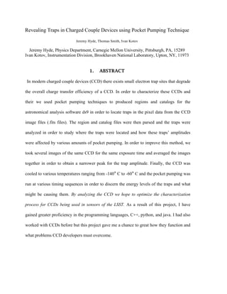
background, each pixel, x-coordinate, y-coordinate, and tile number for each trap.

Fig. 1 Pocket pumping regions shown in ds9 with red rectangles around them

This file can be loaded along with the FITS file into ds9 to show the location of the traps on
the CCD. This was repeated for several files with the same exposure time but with differing
number of pumps.
In PP_trap_analysis.cpp I wrote code that would parse all region files inputted into it
by looking for key words and extracting data such as the location of the trap, amplitude of the
pixels affected by the trap compared to background and which tile it is in. This information
was stored and values such as number of traps per segments and average amplitude were
calculated. The data was then graphed using root’s TGraph and TMultiGraph.
The next step was to try to improve the signal to noise levels by averaging together
multiple exposures of the same image. Multiple exposures were taken one after another and
added to a directory. I then manipulated the PP_trap.cpp code provided by Ivan Kotov to be
able to take an inputted directory instead of just a single file. The files in the directory were
added to a file list. For each file we performed a base line subtraction, which removed the
overscan value from the pixels. After this base line subtraction (BaLiS) was performed on
each image the pixel values were averaged together into one image and analyzed
accordingly. The data taken is saved in the base directory /data2/e2v/112-04 on the lsst2 in
the format seen in Table 1.

Table 1 The data is sorted in the directories above
Directory)Map)for)2014072*4PocketPump)
)
Base)Directory:!/data1/e2v/112*04!
!
!
!
!
!
Directory) Temperature) Exposure)Time) Pocket)Pump)
!
!
!
20140721*
PocketPump!
(5!files!in!
each)!
Temp_*60C! E2! 1000,!2000,!4000,!8000,!12000!
Temp_*80C! E2! 1000,!2000,!4000,!8000,!12000!
!
!
Temp_*100C!
E0.1! 200,!400,!800,!1600,!5000!
E0.5! 1000,!2000,!4000,!8000,!12000!
E2! 1000,!2000,!4000,!8000,!12000!
E4! 1000,!2000,!4000,!8000,!12000!
E16! 1000,!2000,!4000,!8000,!12000!
E32! 1000,!2000,!4000,!8000,!12000!
Temp_*120C! E2! 1000,!2000,!4000,!8000,!12000!
Temp_*140C! E2! 1000,!2000,!4000,!8000,!12000!
Directory! Timing! Temperature! Exposure)
Time!
Pocket)Pump!
!
!
!
20140722*
PocketPump!
(10!files!in!
each)!
T0! ! ! !
T100! ! ! !
T500! ! ! !
T1000! ! ! !
T2000! ! ! !
T4000! ! ! !
T8000! ! ! !
T16000! ! ! !
BiasOn! Temp_*120C! E0.1! 200,!400,!800,!1600,!5000!
E2! 1000,!2000,!4000,!8000,!
12000!
Directory! Folders!
20140724*
PocketPump!
(200!files!in!
each)!
PP23a_10000_E1_T*120!
PP23a_5000_E0.5_T*120!
PP23a_NoPP_E0.5_T*120!

4. POCKET PUMPING DEPENDENCE
The follow data was collected from a CCD exposed for three seconds and pocket pumped
1000,
2000,
3000,
4000,
5000,
6000,
7000,
8000,
9000,
10000,
11000,
12000,
15000,

and
20000
times.

In figure 2 it is easy to see which segments are bad by the shape and scale of the
graphs. The scale of the segments with low traps go up to around 400 or 800 while the bad
segments such as segment 12 (tile 11) goes up to 30000. The shape of the segments with
Number of Pocket Pumps
0 5000 10000 15000 20000 25000
TrapNumber
0
100
200
300
400
Data
Entries 14
Mean x 8071
Mean y 250.6
RMS x 5092
RMS y 103
Data
Entries 14
Mean x 8071
Mean y 250.6
RMS x 5092
RMS y 103
Trap Number (Tile 0)
0 5000 10000 15000 20000 25000
TrapNumber
0
100
200
300
400
Data
Entries 14
Mean x 7769
Mean y 196
RMS x 5161
RMS y 107.8
Data
Entries 14
Mean x 7769
Mean y 196
RMS x 5161
RMS y 107.8
0 5000 10000 15000 20000 25000
TrapNumber
0
100
200
300
Data
Entries 14
Mean x 7769
Mean y 172.2
RMS x 5161
RMS y 94.66
Data
Entries 14
Mean x 7769
Mean y 172.2
RMS x 5161
RMS y 94.66
0 5000 10000 15000 20000 25000
TrapNumber
0
100
200
300
400
Data
Entries 14
Mean x 7769
Mean y 215.2
RMS x 5161
RMS y 110.7
Data
Entries 14
Mean x 7769
Mean y 215.2
RMS x 5161
RMS y 110.7
0 5000 10000 15000 20000 25000
TrapNumber
0
200
400
600
800
Data
Entries 14
Mean x 8071
Mean y 496
RMS x 5092
RMS y 128.9
Data
Entries 14
Mean x 8071
Mean y 496
RMS x 5092
RMS y 128.9
0 5000 10000 15000 20000 25000
TrapNumber
0
200
400
600
Data
Entries 14
Mean x 8071
Mean y 330.9
RMS x 5092
RMS y 167.1
Data
Entries 14
Mean x 8071
Mean y 330.9
RMS x 5092
RMS y 167.1
0 5000 10000 15000 20000 25000
TrapNumber
0
200
400
Data
Entries 14
Mean x 8071
Mean y 224.9
RMS x 5092
RMS y 147.8
Data
Entries 14
Mean x 8071
Mean y 224.9
RMS x 5092
RMS y 147.8
0 5000 10000 15000 20000 25000
TrapNumber
0
200
400
Data
Entries 14
Mean x 7769
Mean y 280.7
RMS x 5161
RMS y 115.3
Data
Entries 14
Mean x 7769
Mean y 280.7
RMS x 5161
RMS y 115.3
0 5000 10000 15000 20000 25000
TrapNumber
0
200
400
600
Data
Entries 14
Mean x 7769
Mean y 310.4
RMS x 5161
RMS y 136.3
Data
Entries 14
Mean x 7769
Mean y 310.4
RMS x 5161
RMS y 136.3
0 5000 10000 15000 20000 25000
TrapNumber
0
200
400
600
Data
Entries 14
Mean x 8071
Mean y 289.9
RMS x 5092
RMS y 155.6
Data
Entries 14
Mean x 8071
Mean y 289.9
RMS x 5092
RMS y 155.6
0 5000 10000 15000 20000 25000
TrapNumber
0
2000
4000
6000
8000
Data
Entries 14
Mean x 7769
Mean y 6001
RMS x 5161
RMS y 365.2
Data
Entries 14
Mean x 7769
Mean y 6001
RMS x 5161
RMS y 365.2
0 5000 10000 15000 20000 25000
TrapNumber
0
10000
20000
30000
Data
Entries 14
Mean x 7769
Mean y 2.314e+04
RMS x 5161
RMS y 1518
Data
Entries 14
Mean x 7769
Mean y 2.314e+04
RMS x 5161
RMS y 1518
0 5000 10000 15000 20000 25000
TrapNumber
0
500
1000
Data
Entries 14
Mean x 7769
Mean y 797.5
RMS x 5161
RMS y 143.1
Data
Entries 14
Mean x 7769
Mean y 797.5
RMS x 5161
RMS y 143.1
0 5000 10000 15000 20000 25000
TrapNumber
0
200
400
600
800
Data
Entries 14
Mean x 7769
Mean y 490.9
RMS x 5161
RMS y 136.9
Data
Entries 14
Mean x 7769
Mean y 490.9
RMS x 5161
RMS y 136.9
0 5000 10000 15000 20000 25000
TrapNumber
0
100
200
300
400
Data
Entries 14
Mean x 7769
Mean y 179.8
RMS x 5161
RMS y 106.6
Data
Entries 14
Mean x 7769
Mean y 179.8
RMS x 5161
RMS y 106.6
0 5000 10000 15000 20000 25000
TrapNumber
0
100
200
300
400
Data
Entries 14
Mean x 7769
Mean y 178.8
RMS x 5161
RMS y 100.6
Data
Entries 14
Mean x 7769
Mean y 178.8
RMS x 5161
RMS y 100.6
Fig. 2 The number of traps in each tile at various pocket pumping levels. Tiles 10 and 11 are the poor segments.

lower number of traps is also much more sigmoidal due to the difficult initially in finding
them a low number of pumps and over pumping, producing the inflexion point. The segments
with a high concentration of traps tend be much flatter possibly due to the ease of finding
traps initially and once again the over pumping at the end.
An interesting thing to note about Fig. 2 is the number of traps found for the 20000
pocket pumping point. We expected it to be on the same level as the 15000 since the pixels
0 5000 10000 15000 20000 25000
AverageAmpitude(a.d.u)
0
500
1000
1500
2000 Data
Entries 14
Mean x 8071
Mean y 250.4
RMS x 5092
RMS y 56.62
Data
Entries 14
Mean x 8071
Mean y 250.4
RMS x 5092
RMS y 56.62
Average Amplitude (Tile 0)
0 5000 10000 15000 20000 25000
0
500
1000
1500
2000 Data
Entries 14
Mean x 7769
Mean y 260.6
RMS x 5161
RMS y 76
Data
Entries 14
Mean x 7769
Mean y 260.6
RMS x 5161
RMS y 76
0 5000 10000 15000 20000 25000
0
500
1000
1500
2000 Data
Entries 14
Mean x 8071
Mean y 231.1
RMS x 5092
RMS y 95.84
Data
Entries 14
Mean x 8071
Mean y 231.1
RMS x 5092
RMS y 95.84
0 5000 10000 15000 20000 25000
0
500
1000
1500
2000 Data
Entries 14
Mean x 8071
Mean y 423.3
RMS x 5092
RMS y 175.7
Data
Entries 14
Mean x 8071
Mean y 423.3
RMS x 5092
RMS y 175.7
0 5000 10000 15000 20000 25000
0
500
1000
1500
2000 Data
Entries 14
Mean x 8071
Mean y 1007
RMS x 5092
RMS y 338.1
Data
Entries 14
Mean x 8071
Mean y 1007
RMS x 5092
RMS y 338.1
0 5000 10000 15000 20000 25000
0
500
1000
1500
2000 Data
Entries 14
Mean x 8071
Mean y 688.1
RMS x 5092
RMS y 257.2
Data
Entries 14
Mean x 8071
Mean y 688.1
RMS x 5092
RMS y 257.2
0 5000 10000 15000 20000 25000
0
500
1000
1500
2000 Data
Entries 14
Mean x 8071
Mean y 232.3
RMS x 5092
RMS y 93.07
Data
Entries 14
Mean x 8071
Mean y 232.3
RMS x 5092
RMS y 93.07
0 5000 10000 15000 20000 25000
0
500
1000
1500
2000 Data
Entries 14
Mean x 8071
Mean y 228.7
RMS x 5092
RMS y 84.14
Data
Entries 14
Mean x 8071
Mean y 228.7
RMS x 5092
RMS y 84.14
0 5000 10000 15000 20000 25000
0
500
1000
1500
2000 Data
Entries 14
Mean x 8071
Mean y 462.7
RMS x 5092
RMS y 142.4
Data
Entries 14
Mean x 8071
Mean y 462.7
RMS x 5092
RMS y 142.4
0 5000 10000 15000 20000 25000
0
500
1000
1500
2000 Data
Entries 14
Mean x 7769
Mean y 565.5
RMS x 5161
RMS y 98.07
Data
Entries 14
Mean x 7769
Mean y 565.5
RMS x 5161
RMS y 98.07
0 5000 10000 15000 20000 25000
0
500
1000
1500
2000 Data
Entries 14
Mean x 8071
Mean y 1435
RMS x 5092
RMS y 523.6
Data
Entries 14
Mean x 8071
Mean y 1435
RMS x 5092
RMS y 523.6
0 5000 10000 15000 20000 25000
0
500
1000
1500
2000 Data
Entries 14
Mean x 8071
Mean y 1291
RMS x 5092
RMS y 493.2
Data
Entries 14
Mean x 8071
Mean y 1291
RMS x 5092
RMS y 493.2
0 5000 10000 15000 20000 25000
0
500
1000
1500
2000 Data
Entries 14
Mean x 8071
Mean y 1134
RMS x 5092
RMS y 377.3
Data
Entries 14
Mean x 8071
Mean y 1134
RMS x 5092
RMS y 377.3
0 5000 10000 15000 20000 25000
0
500
1000
1500
2000 Data
Entries 14
Mean x 8071
Mean y 844
RMS x 5092
RMS y 276.6
Data
Entries 14
Mean x 8071
Mean y 844
RMS x 5092
RMS y 276.6
0 5000 10000 15000 20000 25000
0
500
1000
1500
2000 Data
Entries 14
Mean x 8071
Mean y 252.6
RMS x 5092
RMS y 93.72
Data
Entries 14
Mean x 8071
Mean y 252.6
RMS x 5092
RMS y 93.72
0 5000 10000 15000 20000 25000
0
500
1000
1500
2000 Data
Entries 14
Mean x 8071
Mean y 260
RMS x 5092
RMS y 95.11
Data
Entries 14
Mean x 8071
Mean y 260
RMS x 5092
RMS y 95.11
Fig. 3 The average amplitude of the traps in each segment at various pocket pumping levels.

with very efficient traps would already have been completely depleted. Instead, we see the
number of traps decrease in almost every segment for an unknown reason.
In Fig. 3 we see the graph of the average amplitude of the traps in each segment plotted
against number of pocket pumps. The amplitude was calculated by taking the absolute value
of the difference between the two pixels and dividing the result by the square root of 2. The
bad segments have much high, almost double, average amplitude for their traps than do the
better segments. However, the most intriguing part of this plot is the shape of the curves and
once again, the 20,000 pocket pumping point.
While some of the good segments increase uniformly, others experience a spike at
around 2000 or 3000 before also increasing uniformly. The spiking requires further
investigation but the uniform increase is to be expected to a certain level as the depletion of
the pixels approach 100%. The bad segments on the other hand asymptotically approach a
maximum average amplitude due to the fact that these segments are very inefficient and have
so many more traps then the good segments whose efficiency approaches 1.
Fig. Fig. 4 The amplitude of each trap in each segment at
various pocket pumping levels.

Fig. 5 A plot of each trap at various pocket pumping levels
( (similar to figure 4)
2000 4000 6000 8000 100001200014000160001800020000
TrapAmplitude(a.d.u)
0
200
400
600
800
1000
1200
Traps (Tile 0)
2000 4000 6000 8000 100001200014000160001800020000
0
200
400
600
800
1000
1200
1400
1600
1800
2000
Traps (Tile 1)
2000 4000 6000 8000 100001200014000160001800020000
0
200
400
600
800
1000
1200
Traps (Tile 2)
2000 4000 6000 8000 100001200014000160001800020000
0
500
1000
1500
2000
2500
3000
3500
4000
4500
Traps (Tile 3)
2000 4000 6000 8000 100001200014000160001800020000
0
1000
2000
3000
4000
5000
6000
7000
8000
9000
Traps (Tile 4)
2000 4000 6000 8000 100001200014000160001800020000
0
1000
2000
3000
4000
5000
6000
7000
Traps (Tile 5)
2000 4000 6000 8000 100001200014000160001800020000
0
200
400
600
800
1000
Traps (Tile 6)
2000 4000 6000 8000 100001200014000160001800020000
0
200
400
600
800
1000
1200
Traps (Tile 7)
2000 4000 6000 8000 100001200014000160001800020000
0
200
400
600
800
1000
1200
1400
1600
1800
2000
2200
Traps (Tile 8)
2000 4000 6000 8000 100001200014000160001800020000
0
200
400
600
800
1000
1200
1400
1600
1800
2000
2200
Traps (Tile 9)
2000 4000 6000 8000 100001200014000160001800020000
0
2000
4000
6000
8000
10000
12000
14000
16000
Traps (Tile 10)
2000 4000 6000 8000 100001200014000160001800020000
0
2000
4000
6000
8000
10000
12000
14000
16000
Traps (Tile 11)
2000 4000 6000 8000 100001200014000160001800020000
0
200
400
600
800
1000
1200
1400
1600
1800
2000
2200
2400
Traps (Tile 12)
2000 4000 6000 8000 100001200014000160001800020000
0
1000
2000
3000
4000
5000
6000
7000
Traps (Tile 13)
2000 4000 6000 8000 100001200014000160001800020000
0
200
400
600
800
1000
1200
Traps (Tile 14)
2000 4000 6000 8000 100001200014000160001800020000
0
200
400
600
800
1000
1200
1400
Traps (Tile 15)

The 20,000 pocket pumping level appears to decrease in all segments once again. This
is very noticeable in the bad segments where the 20,000 point jumps down to around a third
of the 15000 level instead of staying at the same level as expected. When looking at the
region file in ds9 I found that the difference between the background and overscan was
around 1,000 at the 20,000 pocket pumping level while it was 3,000 at all other levels.
Whether this 1:3 ratio observed again is correlated with the average amplitude difference has
yet to be determined.
The plot of each trap is shown in its appropriate tile in Fig. 4/5. Fig. 6 and Fig.7 show
zoomed in copies of a relatively good segment (segment 4) and a relatively bad one (segment
12). Most of the traps follow a similar increasing to a certain level and then leveling out
when the pixel the trap is in becomes fully depleted. Some of the noted outliers to this pattern
are the zigzags appearing in many of the tiles. Even the bad segments follow this pattern if to
a higher amplitude as in Fig. 7.
The 20,000 pocket pumping level point is interesting. As can be seen in most tiles and
especially in Fig. 7, many of the traps disappear after the 15,000 point. While this was
expected due to Fig. 2, I expected that it would be some of the lower amplitude traps if any
that would disappear but instead it seems like it is mostly the higher ones that are. Further
investigation is required to determine why certain traps are disappearing.

5. IMAGE AVERAGING
The goal of averaging together images of the same CCD under the same conditions was to
decrease the shot noise to signal ratio. The shot noise causes the pixels to fluctuate around a
mean value; these fluctuations produce a Poisson distribution and an RMS value associated
with the width of the distribution, therefore any decrease in shot noise to signal ratio should
be seen in the RMS value. If the images were independent we would expect the RMS value
Fig. 6 The amplitude of each trap in segment 4 at various
pocket pumping levels
Fig. 7 The amplitude of each trap in segment 12 at various
pocket pumping levels
2000 4000 6000 8000 10000 12000 14000 16000 18000 20000
0
1000
2000
3000
4000
5000
6000
7000
Traps (Tile 5)
2000 4000 6000 8000 10000 12000 14000 16000 18000 20000
0
1000
2000
3000
4000
5000
6000
7000
Traps (Tile 5)
Fig.
8
The
number
of
pixels
at
various
amplitudes

for
a
single
image

Fig.
9
The
number
of
pixels
at
various
amplitudes

for
a
100
images

Am p - BL Histogram ch 1
Entries 1024000
Mean -0.001495
RMS 13.24
Amplitude
-2000 0 2000 4000
1
10
2
10
3
10
4
10
5
10
Entries 1024000
Mean -0.001495
RMS 13.24
Amp - BL Histogram ch 1
Entries 1024000
Mean 0.003924
RMS 13.63
Amplitude
-2000 0 2000 4000
1
10
2
10
3
10
4
10
5
10
Entries 1024000
Mean 0.003924
RMS 13.63
Entries 1024000
Mean -0.00106
RMS 13.73
Amplitude
-2000 0 2000 4000
1
10
2
10
3
10
4
10
5
10
Entries 1024000
Mean -0.00106
RMS 13.73
Amp - BL Histogram ch
Entries1024000
Mean-0.007995
RMS 13.5
Amplitude
-2000 0 2000 4000
1
10
2
10
3
10
4
10
5
10
Entries1024000
Mean-0.007995
RMS 13.5
A mp - B L Histogram ch 5
Entries 1024000
Mean -0.02566
RMS 13.51
Amplitude
-2000 0 2000 4000
1
10
2
10
3
10
4
10
5
10
Entries 1024000
Mean -0.02566
RMS 13.51
Entries 1024000
Mean -0.004712
RMS 13.34
Amplitude
-2000 0 2000 4000
1
10
2
10
3
10
4
10
5
10
Entries 1024000
Mean -0.004712
RMS 13.34
Entries1024000
Mean-0.002156
RMS 13.98
Amplitude
-2000 0 2000 4000
1
10
2
10
3
10
4
10
5
10
Entries1024000
Mean-0.002156
RMS 13.98
A mp - B L Histogram ch 9
Entries 1024000
Mean 0.0009788
RMS 13.42
Amplitude
-200 -100 0 100 200
10
2
10
3
10
4
10
5
10
Entries 1024000
Mean 0.0009788
RMS 13.42
Entries 1024000
Mean 0.03402
RMS 14.87
Amplitude
-2000 0 2000 4000
1
10
2
10
3
10
4
10
5
10
Entries 1024000
Mean 0.03402
RMS 14.87
Entries 1024000
Mean -0.004794
RMS 13.82
Amplitude
-2000 0 2000 4000
1
10
2
10
3
10
4
10
5
10
Entries 1024000
Mean -0.004794
RMS 13.82
Entries 1024000
Mean -0.00352
RMS 14.39
Amplitude
-2000 0 2000 4000
1
10
2
10
3
10
4
10
5
10
Entries 1024000
Mean -0.00352
RMS 14.39
Entries 1024000
Mean 0.004617
RMS 14.08
Amplitude
-2000 0 2000 4000
1
10
2
10
3
10
4
10
5
10
Entries 1024000
Mean 0.004617
RMS 14.08
Entries 1024000
Mean -0.02631
RMS 6.28
Amplitude
-2000 0 2000 4000
1
10
2
10
3
10
4
10
5
10
6
10
Entries 1024000
Mean -0.02631
RMS 6.28
Entries 1024000
Mean 0.001771
RMS 5.592
Amplitude
-2000 0 2000 4000
1
10
2
10
3
10
4
10
5
10
6
10
Entries 1024000
Mean 0.001771
RMS 5.592
Entries 1024000
Mean -6.167e-05
RMS 5.945
Amplitude
-2000 0 2000 4000
1
10
2
10
3
10
4
10
5
10
6
10
Entries 1024000
Mean -6.167e-05
RMS 5.945
-2000
1
10
2
10
3
10
4
10
5
10
6
10
Am
Entries 1024000
Mean -0.003522
RMS 6.544
Amplitude
-2000 0 2000 4000
1
10
2
10
3
10
4
10
5
10
6
10
Entries 1024000
Mean -0.003522
RMS 6.544
Entries 1024000
Mean -0.01175
RMS 6.474
Amplitude
-2000 0 2000 4000
1
10
2
10
3
10
4
10
5
10
6
10
Entries 1024000
Mean -0.01175
RMS 6.474
Amp - BL Histo gram ch 5
Entries 1024000
Mean -0.02484
RMS 6.276
Amplitude
-2000 0 2000 4000
1
10
10
10
10
10
10
Entries 1024000
Mean -0.02484
RMS 6.276
-2000
1
10
2
10
3
10
4
10
5
10
6
10
Am
Entries 1024000
Mean -0.005907
RMS 6.233
Amplitude
-2000 0 2000 4000
1
10
2
10
3
10
4
10
5
10
6
10
Entries 1024000
Mean -0.005907
RMS 6.233
Entries 1024000
Mean-0.0001809
RMS 6.611
Amplitude
-2000 0 2000 4000
1
10
2
10
3
10
4
10
5
10
6
10
Entries 1024000
Mean-0.0001809
RMS 6.611
Entries 1024000
Mean 0.00542
RMS 4.541
Amplitude
-200 -100 0 100 200
1
10
2
10
3
10
4
10
5
10
6
10
Entries 1024000
Mean 0.00542
RMS 4.541
-2000
1
10
2
10
3
10
4
10
5
10
6
10
Am
Entries 1024000
Mean -0.006487
RMS 6.613
Amplitude
-2000 0 2000 4000
1
10
2
10
3
10
4
10
5
10
6
10
Entries 1024000
Mean -0.006487
RMS 6.613
Entries 1024000
Mean -0.003323
RMS 6.594
Amplitude
-2000 0 2000 4000
1
10
2
10
3
10
4
10
5
10
6
10
Entries 1024000
Mean -0.003323
RMS 6.594
Entries 1024000
Mean -0.003325
RMS 6.838
Amplitude
-2000 0 2000 4000
1
10
2
10
3
10
4
10
5
10
6
10
Entries 1024000
Mean -0.003325
RMS 6.838
-2000
1
10
2
10
3
10
4
10
5
10
6
10
Am

to decrease by a factor of the square root of the number of files so if you inputted a directory
with say 100 files it should decrease to around a tenth the original. As can be seen when
comparing Fig. 8 to Fig. 9 this is not the case, While it is true that the RMS value of the
multiple image graph does decrease compared to the RMS value of the single image this
decrease is only around 30% instead of the predicted 10%, this means that there is some issue
most probably some innate correlation between pixels in the same rows or columns.

6. TIMING DEPENDENCE
The
timing
and
speed
of
the
pocket
pumping
affects
the
amplitude
of
the
traps
should

allow
us
to
determine
the
characteristic
emission
time
of
the
trap, τe. As can be seen in
Fig. 10, not only has the amplitude of the traps, with an increase in pocket pumping speed, i.e.
a decrease in the time the trap is in each phase, but the number of traps has also grown. As can
be seen in Fig. 11 there is an increase in the number of traps until around 40 µs per step at
which point it begins to level out. Unlike the number of traps the amplitude of the traps stays
constant. These two facts imply that the best pumping seems to occur when the timing is
around 1 µs or 5 µs per step.

Fig. 10 Images taken when timing was set to 1 µs, 5 µs, 10, µs, 20 µs, 40 µs, 8000 µs
per step at -120° C and 8000 pumps.

7. TEMPERATURE DEPENDENCE
Finally we began to study the temperature dependence of the CCD in hopes of combing what
we found with the timing dependence to determine the energy level of the traps. As can be
seen in Fig. 12 the number of traps found increases with temperature until - 100 ° C at which
point it drops sharply and then keeps dropping at a more moderate rate. This indicates that
the best temperature to run thee CCD at seems to be at hotter temperatures, however, one
must balance this against the dark current which is least at low temperatures. This means that
the optimal temperature for the CCD to function at is about 80 ° C.
Fig. 11 Dependence of the number of traps located with then time
each step takes at -120° C and 8000 pumps.

Timing (microseconds)
0 50 100 150 200
TrapNumber
0
2000
4000
6000
8000
10000 Data
Entries 7
Mean x 49.33
Mean y 7672
RMS x 56.46
RMS y 849.8
Data
Entries 7
Mean x 49.33
Mean y 7672
RMS x 56.46
RMS y 849.8
Trap Number

8. CONCLUSION
The novel trap identification technique has been developed. This technique has been used
to analyze pocket pumped images obtained with CCD 250 at various temperatures, timings
and pocket pumping levels. For the 113-03 CCD the optimal temperatures seems to be at -80°
C. In the future by using the timing dependence we can calculate the τe, which in turn can be
used with the temperature dependence to determine the energy level of the trap, and hint at
what imperfection in the crystal structure of the CCD caused it.

9. AKNOWLEGEMENTS
This
project
was
supported
in
part
by
the
U.S.
Department
of
Energy,
Office
of

Science,
Office
of
Workforce
Development
for
Teachers
and
Scientists
(WDTS)
under

the
Science
Undergraduate
Laboratory
Internship
Program
(SULI).

Temperature (C)
-140 -120 -100 -80 -60
TrapNumber
0
2000
4000
6000
Data
Entries 5
Mean x -100
Mean y 2776
RMS x 28.28
RMS y 1946
Data
Entries 5
Mean x -100
Mean y 2776
RMS x 28.28
RMS y 1946
Trap Number
Fig. 12 Dependence of the number of traps located with then temperature of the
CCD taken with an exposure of 2 seconds and 4000 pumps.

Hall,
David
J.;
Murray,
Neil
J.;
Holland,
Andrew
D.;
Gow,
Jason;
Clarke,
Andrew
and

Burt,
David
(2014).
Determination
of
in
situ
trap
properties
in
CCDs
using
a
“single-‐
trap
pumping”
technique.
IEEE
Transactions
on
Nuclear
Science
(In
press).

SULI HYDE J Report

Recommended

Recommended

More Related Content

What's hot

What's hot (11)

Viewers also liked

Viewers also liked (11)

Similar to SULI HYDE J Report

Similar to SULI HYDE J Report (20)

SULI HYDE J Report