
Recommended
More Related Content
Similar to Mining Big Data for Insights and Predictions
Similar to Mining Big Data for Insights and Predictions (20)
More from ImXaib
More from ImXaib (20)
Recently uploaded
Recently uploaded (20)
Mining Big Data for Insights and Predictions
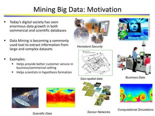
- 1. Mining Big Data: Motivation Today’s digital society has seen enormous data growth in both commercial and scientific databases Data Mining is becoming a commonly used tool to extract information from large and complex datasets Examples: Helps provide better customer service in business/commercial setting Helps scientists in hypothesis formation Computational Simulations Business Data Sensor Networks Geo-spatial data Homeland Security Scientific Data
- 2. Data Mining for Life and Health Sciences Recent technological advances are helping to generate large amounts of both medical and genomic data • High-throughput experiments/techniques - Gene and protein sequences - Gene-expression data - Biological networks and phylogenetic profiles • Electronic Medical Records - IBM-Mayo clinic partnership has created a DB of 5 million patients - Single Nucleotides Polymorphisms (SNPs) Data mining offers potential solution for analysis of large-scale data • Automated analysis of patients history for customized treatment • Prediction of the functions of anonymous genes • Identification of putative binding sites in protein structures for drugs/chemicals discovery Protein Interaction Network
- 3. • Draws ideas from machine learning/AI, pattern recognition, statistics, and database systems • Traditional Techniques may be unsuitable due to – Enormity of data – High dimensionality of data – Heterogeneous, distributed nature of data Origins of Data Mining Machine Learning/ Pattern Recognition Statistics/ AI Data Mining Database systems
- 4. Data Mining as Part of the Knowledge Discovery Process
- 5. Data Mining Tasks... Tid Refund Marital Status Taxable Income Cheat 1 Yes Single 125K No 2 No Married 100K No 3 No Single 70K No 4 Yes Married 120K No 5 No Divorced 95K Yes 6 No Married 60K No 7 Yes Divorced 220K No 8 No Single 85K Yes 9 No Married 75K No 10 No Single 90K Yes 11 No Married 60K No 12 Yes Divorced 220K No 13 No Single 85K Yes 14 No Married 75K No 15 No Single 90K Yes 10 Milk Data
- 6. August 21, 2022 Data Mining: Concepts and Techniques 6 Data Mining Functions: Generalization • Materials to be covered in Chapters 2-4 • Information integration and data warehouse construction – Data cleaning, transformation, integration, and multidimensional data model • Data cube technology – Scalable methods for computing (i.e., materializing) multidimensional aggregates – OLAP (online analytical processing) • Multidimensional concept description: Characterization and discrimination – Generalize, summarize, and contrast data characteristics, e.g., dry vs. wet regions
- 7. August 21, 2022 Data Mining: Concepts and Techniques 7 Data Mining Functions: Association and Correlation • Frequent patterns (or frequent itemsets) – What items are frequently purchased together in your Walmart? • Association, correlation vs. causality – A typical association rule • Diaper Beer [0.5%, 75%] (support, confidence) – Are strongly associated items also strongly correlated? • How to mine such patterns and rules efficiently in large datasets? • How to use such patterns for classification, clustering, and other applications?
- 8. August 21, 2022 Data Mining: Concepts and Techniques 8 Data Mining Functions: Classification and Prediction • Classification and prediction – Construct models (functions) based on some training examples – Describe and distinguish classes or concepts for future prediction • E.g., classify countries based on (climate), or classify cars based on (gas mileage) – Predict some unknown or missing numerical values • Typical methods – Decision trees, naïve Bayesian classification, support vector machines, neural networks, rule-based classification, pattern-based classification, logistic regression, … • Typical applications: – Credit card fraud detection, direct marketing, classifying stars, diseases, web-pages, …
- 9. August 21, 2022 Data Mining: Concepts and Techniques 9 Data Mining Functions: Cluster and Outlier Analysis • Cluster analysis – Unsupervised learning (i.e., Class label is unknown) – Group data to form new categories (i.e., clusters), e.g., cluster houses to find distribution patterns – Principle: Maximizing intra-class similarity & minimizing interclass similarity – Many methods and applications • Outlier analysis – Outlier: A data object that does not comply with the general behavior of the data – Noise or exception? ― One person’s garbage could be another person’s treasure – Methods: by product of clustering or regression analysis, … – Useful in fraud detection, rare events analysis
- 10. August 21, 2022 Data Mining: Concepts and Techniques 10 Data Mining Functions: Trend and Evolution Analysis • Sequence, trend and evolution analysis – Trend and deviation analysis: e.g., regression – Sequential pattern mining • e.g., first buy digital camera, then large SD memory cards – Periodicity analysis – Motifs, time-series, and biological sequence analysis • Approximate and consecutive motifs – Similarity-based analysis • Mining data streams – Ordered, time-varying, potentially infinite, data streams
- 11. August 21, 2022 Data Mining: Concepts and Techniques 11 Data Mining Functions:Structure and Network Analysis • Graph mining – Finding frequent subgraphs (e.g., chemical compounds), trees (XML), substructures (web fragments) • Information network analysis – Social networks: actors (objects, nodes) and relationships (edges) • e.g., author networks in CS, terrorist networks – Multiple heterogeneous networks • A person could be multiple information networks: friends, family, classmates, … – Links carry a lot of semantic information: Link mining • Web mining – Web is a big information network: from PageRank to Google – Analysis of Web information networks • Web community discovery, opinion mining, usage mining, …
- 13. General Approach for Building a Classification Model Test Set Training Set Model Learn Classifier Tid Employed Level of Education # years at present address Credit Worthy 1 Yes Graduate 5 Yes 2 Yes High School 2 No 3 No Undergrad 1 No 4 Yes High School 10 Yes … … … … … 10 Tid Employed Level of Education # years at present address Credit Worthy 1 Yes Undergrad 7 ? 2 No Graduate 3 ? 3 Yes High School 2 ? … … … … … 10
- 14. • Predicting tumor cells as benign or malignant • Classifying secondary structures of protein as alpha-helix, beta-sheet, or random coil • Predicting functions of proteins • Classifying credit card transactions as legitimate or fraudulent • Categorizing news stories as finance, weather, entertainment, sports, etc • Identifying intruders in the cyberspace Examples of Classification Task
- 15. Commonly Used Classification Models • Base Classifiers – Decision Tree based Methods – Rule-based Methods – Nearest-neighbor – Neural Networks – Naïve Bayes and Bayesian Belief Networks – Support Vector Machines • Ensemble Classifiers – Boosting, Bagging, Random Forests
- 16. Tid Employed Level of Education # years at present address Credit Worthy 1 Yes Graduate 5 Yes 2 Yes High School 2 No 3 No Undergrad 1 No 4 Yes High School 10 Yes … … … … … 10 Class Model for predicting credit worthiness Employed No Education Number of years No Yes Graduate { High school, Undergrad } Yes No > 7 yrs < 7 yrs Yes Classification Model: Decision Tree
- 17. Constructing a Decision Tree 10 Tid Employed Level of Education # years at present address Credit Worthy 1 Yes Graduate 5 Yes 2 Yes High School 2 No 3 No Undergrad 1 No 4 Yes High School 10 Yes 5 Yes Graduate 2 No 6 No High School 2 No 7 Yes Undergrad 3 No 8 Yes Graduate 8 Yes 9 Yes High School 4 Yes 10 No Graduate 1 No Employed Worthy: 4 Not Worthy: 3 Yes 10 Tid Employed Level of Education # years at present address Credit Worthy 1 Yes Graduate 5 Yes 2 Yes High School 2 No 3 No Undergrad 1 No 4 Yes High School 10 Yes 5 Yes Graduate 2 No 6 No High School 2 No 7 Yes Undergrad 3 No 8 Yes Graduate 8 Yes 9 Yes High School 4 Yes 10 No Graduate 1 No No Worthy: 0 Not Worthy: 3 10 Tid Employed Level of Education # years at present address Credit Worthy 1 Yes Graduate 5 Yes 2 Yes High School 2 No 3 No Undergrad 1 No 4 Yes High School 10 Yes 5 Yes Graduate 2 No 6 No High School 2 No 7 Yes Undergrad 3 No 8 Yes Graduate 8 Yes 9 Yes High School 4 Yes 10 No Graduate 1 No Graduate High School/ Undergrad Worthy: 2 Not Worthy: 2 Education Worthy: 2 Not Worthy: 4 Key Computation Worthy Not Worthy 4 3 0 3 Employed = Yes Employed = No 10 Tid Employed Level of Education # years at present address Credit Worthy 1 Yes Graduate 5 Yes 2 Yes High School 2 No 3 No Undergrad 1 No 4 Yes High School 10 Yes 5 Yes Graduate 2 No 6 No High School 2 No 7 Yes Undergrad 3 No 8 Yes Graduate 8 Yes 9 Yes High School 4 Yes 10 No Graduate 1 No Worthy: 4 Not Worthy: 3 Yes No Worthy: 0 Not Worthy: 3 Employed
- 18. Constructing a Decision Tree Employed = Yes Employed = No 10 Tid Employed Level of Education # years at present address Credit Worthy 1 Yes Graduate 5 Yes 2 Yes High School 2 No 3 No Undergrad 1 No 4 Yes High School 10 Yes 5 Yes Graduate 2 No 6 No High School 2 No 7 Yes Undergrad 3 No 8 Yes Graduate 8 Yes 9 Yes High School 4 Yes 10 No Graduate 1 No 10 Tid Employed Level of Education # years at present address Credit Worthy 1 Yes Graduate 5 Yes 2 Yes High School 2 No 4 Yes High School 10 Yes 5 Yes Graduate 2 No 7 Yes Undergrad 3 No 8 Yes Graduate 8 Yes 9 Yes High School 4 Yes 10 Tid Employed Level of Education # years at present address Credit Worthy 3 No Undergrad 1 No 6 No High School 2 No 10 No Graduate 1 No
- 19. Classification Errors • Training errors (apparent errors) – Errors committed on the training set • Test errors – Errors committed on the test set • Generalization errors – Expected error of a model over random selection of records from same distribution
- 20. Example Data Set Two class problem: + : 5200 instances • 5000 instances generated from a Gaussian centered at (10,10) • 200 noisy instances added o : 5200 instances • Generated from a uniform distribution 10 % of the data used for training and 90% of the data used for testing
- 21. Design Issues of Decision Tree Induction • How should training records be split? – Method for specifying test condition • depending on attribute types – Measure for evaluating the goodness of a test condition • How should the splitting procedure stop? – Stop splitting if all the records belong to the same class or have identical attribute values – Early termination
- 22. Model Overfitting Underfitting: when model is too simple, both training and test errors are large Overfitting: when model is too complex, training error is small but test error is large
- 23. Model Overfitting Using twice the number of data instances • If training data is under-representative, testing errors increase and training errors decrease on increasing number of nodes • Increasing the size of training data reduces the difference between training and testing errors at a given number of nodes
- 24. Reasons for Model Overfitting • Presence of Noise • Lack of Representative Samples • Multiple Comparison Procedure
- 25. Notes on Overfitting • Overfitting results in decision trees that are more complex than necessary • Training error does not provide a good estimate of how well the tree will perform on previously unseen records • Need ways for incorporating model complexity into model development
- 26. Clustering Algorithms • K-means and its variants • Hierarchical clustering • Other types of clustering
- 27. K-means Clustering • Partitional clustering approach • Number of clusters, K, must be specified • Each cluster is associated with a centroid (center point) • Each point is assigned to the cluster with the closest centroid • The basic algorithm is very simple
- 28. Example of K-means Clustering -2 -1.5 -1 -0.5 0 0.5 1 1.5 2 0 0.5 1 1.5 2 2.5 3 x y Iteration 1 -2 -1.5 -1 -0.5 0 0.5 1 1.5 2 0 0.5 1 1.5 2 2.5 3 x y Iteration 2 -2 -1.5 -1 -0.5 0 0.5 1 1.5 2 0 0.5 1 1.5 2 2.5 3 x y Iteration 3 -2 -1.5 -1 -0.5 0 0.5 1 1.5 2 0 0.5 1 1.5 2 2.5 3 x y Iteration 4 -2 -1.5 -1 -0.5 0 0.5 1 1.5 2 0 0.5 1 1.5 2 2.5 3 x y Iteration 5 -2 -1.5 -1 -0.5 0 0.5 1 1.5 2 0 0.5 1 1.5 2 2.5 3 x y Iteration 6
- 29. K-means Clustering – Details • The centroid is (typically) the mean of the points in the cluster • Initial centroids are often chosen randomly – Clusters produced vary from one run to another • ‘Closeness’ is measured by Euclidean distance, cosine similarity, correlation, etc • Complexity is O( n * K * I * d ) – n = number of points, K = number of clusters, I = number of iterations, d = number of attributes
- 30. Evaluating K-means Clusters • Most common measure is Sum of Squared Error (SSE) – For each point, the error is the distance to the nearest cluster – To get SSE, we square these errors and sum them • x is a data point in cluster Ci and mi is the representative point for cluster Ci – Given two sets of clusters, we prefer the one with the smallest error – One easy way to reduce SSE is to increase K, the number of clusters K i C x i i x m dist SSE 1 2 ) , (
- 31. Two different K-means Clusterings -2 -1.5 -1 -0.5 0 0.5 1 1.5 2 0 0.5 1 1.5 2 2.5 3 x y -2 -1.5 -1 -0.5 0 0.5 1 1.5 2 0 0.5 1 1.5 2 2.5 3 x y Sub-optimal Clustering -2 -1.5 -1 -0.5 0 0.5 1 1.5 2 0 0.5 1 1.5 2 2.5 3 x y Optimal Clustering Original Points
- 32. Limitations of K-means • K-means has problems when clusters are of differing – Sizes – Densities – Non-globular shapes • K-means has problems when the data contains outliers.
- 33. Limitations of K-means: Differing Sizes Original Points K-means (3 Clusters)
- 34. Limitations of K-means: Differing Density Original Points K-means (3 Clusters)
- 35. Limitations of K-means: Non-globular Shapes Original Points K-means (2 Clusters)
- 36. Hierarchical Clustering • Produces a set of nested clusters organized as a hierarchical tree • Can be visualized as a dendrogram – A tree like diagram that records the sequences of merges or splits 1 2 3 4 5 6 1 2 3 4 5 3 6 2 5 4 1 0 0.05 0.1 0.15 0.2
- 37. Strengths of Hierarchical Clustering • Do not have to assume any particular number of clusters – Any desired number of clusters can be obtained by ‘cutting’ the dendrogram at the proper level • They may correspond to meaningful taxonomies – Example in biological sciences (e.g., animal kingdom, phylogeny reconstruction, …)
- 38. Hierarchical Clustering • Two main types of hierarchical clustering – Agglomerative: • Start with the points as individual clusters • At each step, merge the closest pair of clusters until only one cluster (or k clusters) left – Divisive: • Start with one, all-inclusive cluster • At each step, split a cluster until each cluster contains a point (or there are k clusters) • Traditional hierarchical algorithms use a similarity or distance matrix – Merge or split one cluster at a time
- 39. Agglomerative Clustering Algorithm • More popular hierarchical clustering technique • Basic algorithm is straightforward 1. Compute the proximity matrix 2. Let each data point be a cluster 3. Repeat 4. Merge the two closest clusters 5. Update the proximity matrix 6. Until only a single cluster remains • Key operation is the computation of the proximity of two clusters – Different approaches to defining the distance between clusters distinguish the different algorithms
- 40. Starting Situation • Start with clusters of individual points and a proximity matrix p1 p3 p5 p4 p2 p1 p2 p3 p4 p5 . . . . . . Proximity Matrix ... p1 p2 p3 p4 p9 p10 p11 p12
- 41. Intermediate Situation • After some merging steps, we have some clusters C1 C4 C2 C5 C3 C2 C1 C1 C3 C5 C4 C2 C3 C4 C5 Proximity Matrix ... p1 p2 p3 p4 p9 p10 p11 p12
- 42. Intermediate Situation • We want to merge the two closest clusters (C2 and C5) and update the proximity matrix. C1 C4 C2 C5 C3 C2 C1 C1 C3 C5 C4 C2 C3 C4 C5 Proximity Matrix ... p1 p2 p3 p4 p9 p10 p11 p12
- 43. After Merging • The question is “How do we update the proximity matrix?” C1 C4 C2 U C5 C3 ? ? ? ? ? ? ? C2 U C5 C1 C1 C3 C4 C2 U C5 C3 C4 Proximity Matrix ... p1 p2 p3 p4 p9 p10 p11 p12
- 44. How to Define Inter-Cluster Distance p1 p3 p5 p4 p2 p1 p2 p3 p4 p5 . . . . . . Similarity? • MIN • MAX • Group Average • Distance Between Centroids • Other methods driven by an objective function – Ward’s Method uses squared error Proximity Matrix
- 45. How to Define Inter-Cluster Similarity p1 p3 p5 p4 p2 p1 p2 p3 p4 p5 . . . . . . Proximity Matrix • MIN • MAX • Group Average • Distance Between Centroids • Other methods driven by an objective function – Ward’s Method uses squared error
- 46. How to Define Inter-Cluster Similarity p1 p3 p5 p4 p2 p1 p2 p3 p4 p5 . . . . . . Proximity Matrix • MIN • MAX • Group Average • Distance Between Centroids • Other methods driven by an objective function – Ward’s Method uses squared error
- 47. How to Define Inter-Cluster Similarity p1 p3 p5 p4 p2 p1 p2 p3 p4 p5 . . . . . . Proximity Matrix • MIN • MAX • Group Average • Distance Between Centroids • Other methods driven by an objective function – Ward’s Method uses squared error
- 48. How to Define Inter-Cluster Similarity p1 p3 p5 p4 p2 p1 p2 p3 p4 p5 . . . . . . Proximity Matrix • MIN • MAX • Group Average • Distance Between Centroids • Other methods driven by an objective function – Ward’s Method uses squared error
- 49. Other Types of Cluster Algorithms • Hundreds of clustering algorithms • Some clustering algorithms – K-means – Hierarchical – Statistically based clustering algorithms • Mixture model based clustering – Fuzzy clustering – Self-organizing Maps (SOM) – Density-based (DBSCAN) • Proper choice of algorithms depends on the type of clusters to be found, the type of data, and the objective
- 50. Cluster Validity • For supervised classification we have a variety of measures to evaluate how good our model is – Accuracy, precision, recall • For cluster analysis, the analogous question is how to evaluate the “goodness” of the resulting clusters? • But “clusters are in the eye of the beholder”! • Then why do we want to evaluate them? – To avoid finding patterns in noise – To compare clustering algorithms – To compare two sets of clusters – To compare two clusters
- 51. Clusters found in Random Data 0 0.2 0.4 0.6 0.8 1 0 0.1 0.2 0.3 0.4 0.5 0.6 0.7 0.8 0.9 1 x y Random Points 0 0.2 0.4 0.6 0.8 1 0 0.1 0.2 0.3 0.4 0.5 0.6 0.7 0.8 0.9 1 x y K-means 0 0.2 0.4 0.6 0.8 1 0 0.1 0.2 0.3 0.4 0.5 0.6 0.7 0.8 0.9 1 x y DBSCAN 0 0.2 0.4 0.6 0.8 1 0 0.1 0.2 0.3 0.4 0.5 0.6 0.7 0.8 0.9 1 x y Complete Link
- 52. • Distinguishing whether non-random structure actually exists in the data • Comparing the results of a cluster analysis to externally known results, e.g., to externally given class labels • Evaluating how well the results of a cluster analysis fit the data without reference to external information • Comparing the results of two different sets of cluster analyses to determine which is better • Determining the ‘correct’ number of clusters Different Aspects of Cluster Validation
- 53. • Order the similarity matrix with respect to cluster labels and inspect visually. Using Similarity Matrix for Cluster Validation 0 0.2 0.4 0.6 0.8 1 0 0.1 0.2 0.3 0.4 0.5 0.6 0.7 0.8 0.9 1 x y Points Points 20 40 60 80 100 10 20 30 40 50 60 70 80 90 100 Similarity 0 0.1 0.2 0.3 0.4 0.5 0.6 0.7 0.8 0.9 1
- 54. Using Similarity Matrix for Cluster Validation • Clusters in random data are not so crisp Points Points 20 40 60 80 100 10 20 30 40 50 60 70 80 90 100 Similarity 0 0.1 0.2 0.3 0.4 0.5 0.6 0.7 0.8 0.9 1 DBSCAN 0 0.2 0.4 0.6 0.8 1 0 0.1 0.2 0.3 0.4 0.5 0.6 0.7 0.8 0.9 1 x y
- 55. Points Points 20 40 60 80 100 10 20 30 40 50 60 70 80 90 100 Similarity 0 0.1 0.2 0.3 0.4 0.5 0.6 0.7 0.8 0.9 1 Using Similarity Matrix for Cluster Validation • Clusters in random data are not so crisp K-means 0 0.2 0.4 0.6 0.8 1 0 0.1 0.2 0.3 0.4 0.5 0.6 0.7 0.8 0.9 1 x y
- 56. Using Similarity Matrix for Cluster Validation • Clusters in random data are not so crisp 0 0.2 0.4 0.6 0.8 1 0 0.1 0.2 0.3 0.4 0.5 0.6 0.7 0.8 0.9 1 x y Points Points 20 40 60 80 100 10 20 30 40 50 60 70 80 90 100 Similarity 0 0.1 0.2 0.3 0.4 0.5 0.6 0.7 0.8 0.9 1 Complete Link
- 57. • Numerical measures that are applied to judge various aspects of cluster validity, are classified into the following three types of indices. – External Index: Used to measure the extent to which cluster labels match externally supplied class labels. • Entropy – Internal Index: Used to measure the goodness of a clustering structure without respect to external information. • Sum of Squared Error (SSE) – Relative Index: Used to compare two different clusterings or clusters. • Often an external or internal index is used for this function, e.g., SSE or entropy • For futher details please see “Introduction to Data Mining”, Chapter 8. – http://www-users.cs.umn.edu/~kumar/dmbook/ch8.pdf Measures of Cluster Validity
- 59. Association Analysis • Given a set of records, find dependency rules which will predict occurrence of an item based on occurrences of other items in the record • Applications – Marketing and Sales Promotion – Supermarket shelf management – Traffic pattern analysis (e.g., rules such as "high congestion on Intersection 58 implies high accident rates for left turning traffic") TID Items 1 Bread, Coke, Milk 2 Beer, Bread 3 Beer, Coke, Diaper, Milk 4 Beer, Bread, Diaper, Milk 5 Coke, Diaper, Milk Rules Discovered: {Milk} --> {Coke} (s=0.6, c=0.75) {Diaper, Milk} --> {Beer} (s=0.4, c=0.67) ons transacti Total Y and X contain that ons transacti # s Support, X contain that ons transacti # Y and X contain that ons transacti # c , Confidence
- 60. Association Rule Mining Task • Given a set of transactions T, the goal of association rule mining is to find all rules having – support ≥ minsup threshold – confidence ≥ minconf threshold • Brute-force approach: Two Steps – Frequent Itemset Generation • Generate all itemsets whose support minsup – Rule Generation • Generate high confidence rules from each frequent itemset, where each rule is a binary partitioning of a frequent itemset • Frequent itemset generation is computationally expensive
- 61. Efficient Pruning Strategy (Ref: Agrawal & Srikant 1994) If an itemset is infrequent, then all of its supersets must also be infrequent null AB AC AD AE BC BD BE CD CE DE A B C D E ABC ABD ABE ACD ACE ADE BCD BCE BDE CDE ABCD ABCE ABDE ACDE BCDE ABCDE Found to be Infrequent null AB AC AD AE BC BD BE CD CE DE A B C D E ABC ABD ABE ACD ACE ADE BCD BCE BDE CDE ABCD ABCE ABDE ACDE BCDE ABCDE null AB AC AD AE BC BD BE CD CE DE A B C D E ABC ABD ABE ACD ACE ADE BCD BCE BDE CDE ABCD ABCE ABDE ACDE BCDE ABCDE Pruned supersets
- 62. Illustrating Apriori Principle Item Count Bread 4 Coke 2 Milk 4 Beer 3 Diaper 4 Eggs 1 Itemset Count {Bread,Milk} 3 {Bread,Beer} 2 {Bread,Diaper} 3 {Milk,Beer} 2 {Milk,Diaper} 3 {Beer,Diaper} 3 Itemset Count {Bread,Milk,Diaper} 3 Items (1-itemsets) Pairs (2-itemsets) (No need to generate candidates involving Coke or Eggs) Triplets (3-itemsets) Minimum Support = 3 If every subset is considered, 6C1 + 6C2 + 6C3 = 41 With support-based pruning, 6 + 6 + 1 = 13