ABSTRACT: An inventory system is considered with trended demand which is assumed to be a function of price and time dependent quadratic demand. For minimizing the total cost of the inventory system, it is assumed that the deterioration rate is constant and the supplier offers the retailer a credit period to settle the account of the procurement units. To solve the model it is further assumed that shortages are not allowed. Salvage value is also considered and observed its effect on the total cost. A numerical example is given to test the strength of the model. Critical parameters are identified by studying the sensitivity of the system.

1. International
OPEN ACCESS Journal
Of Modern Engineering Research (IJMER)
| IJMER | ISSN: 2249–6645 | www.ijmer.com | Vol. 7 | Iss. 1 | Jan. 2017 | 23 |
A Deterministic Inventory Model for Perishable Items with Price
Sensitive Quadratic Time Dependent Demand Under Trade
Credit Policy
R. Venkateswarlu1,*
, M. S. Reddy2
*
Gitam School Of International Business
Gitam University, Visakhapatnam, India
**
Bvsr Engineering College, Chimakurthy, India
I. INTRODUCTION
In modern business, it is well known that ‘trade credit policy’ is the most effective way of a supplier to
encourage retailer to buy more goods and to attract more retailers. Trade credit can also be used as a multi-
faceted marketing management (or relationship management) tool which gives some information to the market
or to a buyer about the firm or its products or its future plans. The EOQ model developed by Wilson was based
on the assumption that the retailer will pay for the items as soon as it is received by the system. In reality the
supplier may offer some credit period to the retailer to settle the accounts in a reasonable time period. Thus the
delay in payment can be treated as a kind of price discount to the retailer.
Haley and Higgins (1973) studied the relationship between inventory policy and credit policy in the
context of the classical lot size model. Chapman et al. (1984) developed an economic order quantity model
which considers possible credit periods allowable by suppliers. This model is shown to be very sensitive to the
length of the permissible credit period and to the relationship between the credit period and inventory level.
Davis and Gaither (1985) developed optimal order quantities for firms that are offered a onetime opportunity to
delay payment for an order of a commodity. A mathematical model is developed by Goyal (1985) when supplier
announces credit period in settling the account, so that no interest charges are payable from the outstanding
amount if the account is settled with in the allowable delay period. Aggarwal and Jaggi (1995) developed
mathematical model for deteriorating inventories for which supplier allowed certain fixed period to settle the
account. Shah et al. (1988) extended the above model by allowing shortages. Mandal and Phaujdar (1989a, b)
have studied Goyal (1985) model by including interest earned from the sales revenue on the stock remaining
beyond the settlement period. Carlson and Rousseau (1989) examined EOQ under date terms supplier credit by
partitioning carrying cost into financial cost and variable holding costs. Chung and Huang (2003) extended
Goyal (1985) model when replenishment rate is finite.
Dallenbach (1986, 1988), Ward and Chapman (1987), Chapman and Ward (1988) argued that the usual
assumptions as to the incidence and the value of the inventory investment opportunity cost made by the
traditional inventory theory are correct and also established that if trade credit surplus is taken into account, the
optimal ordering quantities decreases rather than increase. Chung (1998) established the convexity of the total
annual variable cost function for optimal economic order quantity under conditions of permissible delay in
payments. Jamal et al. (2000) discussed the problem in which the retailer can pay the supplier either at the end
of credit period or later incurring interest charges on the unpaid balance for the overdue period. Sarker et al.
(2001) obtained optimal payment time under permissible delay in payments when units in an inventory are
subject to deterioration. Abadand Jaggi (2003) considered the seller-buyer channel in which the end demand is
price sensitive and the suppler offers trade credit to the buyer. Shinn and Hwang (2003) dealt with the problem
of determining the retailer’s optimal price and order size simultaneously under the condition of order size
dependent delay in payments. It is assumed that the length of the credit period is a function of the retailer’s
ABSTRACT: An inventory system is considered with trended demand which is assumed to be a
function of price and time dependent quadratic demand. For minimizing the total cost of the inventory
system, it is assumed that the deterioration rate is constant and the supplier offers the retailer a credit
period to settle the account of the procurement units. To solve the model it is further assumed that
shortages are not allowed. Salvage value is also considered and observed its effect on the total cost. A
numerical example is given to test the strength of the model. Critical parameters are identified by
studying the sensitivity of the system.
Keywords: Price sensitive, Quadratic demand, Weibull, holding cost, inventory model, credit policy.

2. A Deterministic Inventory Model for Perishable Items with Price Sensitive...
| IJMER | ISSN: 2249–6645 | www.ijmer.com | Vol. 7 | Iss. 1 | Jan. 2017 | 24 |
order size and also the demand rate is a function of the selling price. Chung et al. (2005) determined the
economic order quantity under conditions of permissible delay in payments where the delay in payments
depends on the quantity ordered when the order quantity is less than the quantity at which the delay in payments
is permitted, the payment for the item must be made immediately. Otherwise, the fixed credit period is allowed.
Huang (2007) examined optimal retailer’s replenishment decisions in the EOQ model under two levels of trade
credit policy by assuming that the supplier would offer the retailer partially permissible delay in payments
when the order quantity is smaller than a predetermined quantity. Tenget. al. (2007) derived retailer’s optimal
ordering policies with trade credit financing.
In this paper, section-2 gives some usual assumptions and notations to develop the mathematical
model. Section-3 contains the formulation and solution of the model. Section- 3.1 contains the offered credit
period is less than or equal to the cycle time i.e., case-1. A numerical example is given in section-3.1.1 for case-
1. Section-3.2 contains the offered credit period is greater than to the cycle time i.e., case-2. A numerical
example is given in section-3.2.1 for case-2. Section-4 contains the sensitive analysis. And finally the
conclusions are discussed in section-5.
II. ASSUMPTIONS AND NOTATIONS
The following assumptions are used to develop the model:
 The system deal with a single item
 The demand rate R(p,t) is a function of price and time dependent quadratic demand
 θ )10(  is the constant rate of deterioration.
 The replenishment rate is infinite.
 The lead time is zero and shortages are not allowed.
 The salvage value, cp )10(  is associated to deteriorated units during the cycle time. Here cp is the
purchase cost of an item.
The following notations are used to develop the model:
 The Demand rate )(tR at time t is assumed to be

 pctbtatpR )1(),( 2
10,0  ba , c < b
and η> 1. Here ‘a’ is a constant demand rate, ‘b’ is the rate of change of the demand and ‘c’ is the
acceleration of demand rate. ‘p’ is the retail price and ‘η’ is price mark up.
 A is the ordering cost per order.
 p is the selling price per unit
 Q(t) is the ordering quantity at time t=0
 his per unit holding cost excluding interest charges per unit per year.
 Ie is the interest earned per year.
 Icis the interest charged per stocks per year.
 M is the permissible delay in settling the accounts, 0<M<1.
 T is the interval between two successive orders
 TC (T, p) is the total cost per unit time.
III. FORMULATION AND SOLUTION OF THE MODEL
Let I(t) be the inventory level at time t ( Tt 0 ). The inventory depletes due to deterioration
and the demand, and then the differential equation which describes the inventory level at time t is given by
TttpRtI
dt
tdI
 0),,()(
)(
 (1)
where

 pctbtatpR )1(),( 2
with the following boundary conditions
(i) I(T) = 0 when t = T, and (ii) I(0) = Q. (2)
The solution of equation (6.1) using the boundary condition I(T) = 0 is given by
  


















 









 
3
)(
2
)(
)(
4
))((
3
))((
2
))((
)(
)()( 3322
443322
tTctTb
tTt
tTctTcbtTb
tT
aptI



(3)

3. A Deterministic Inventory Model for Perishable Items with Price Sensitive...
| IJMER | ISSN: 2249–6645 | www.ijmer.com | Vol. 7 | Iss. 1 | Jan. 2017 | 25 |
where we take series expansion and ignored the second and higher powers of θ as θ is small.
Since I(0) = Q, we obtain










 
4
))((
3
))((
2
))((
)(
432
TcTcbTb
TapQ

(4)
The Ordering cost is given by
OC = A (5)
The number of units that deteriorate during one cycle is given by






 
3
2
2432
)(),()(
32432
cTbTTcTbT
apTTpRQTD

(6)
The cost due to deterioration is given by






 
3
2
2432
)()(.
32432
cTbTTcTbT
apPTDPCD cc

(7)
wherePcis the cost per unit time.
The salvage value is given by






 
3
2
2432
)(.
32432
cTbTTcTbT
apPCDSV c

 
(8)
The inventory holding cost during the cycle is given by





 
  120
121540304060
)(
543432
0
TcTbTcTbTT
hdttIhIHC
T

(9)
We now calculate the total cost of the inventory system in the following two cases:
3.1 Case 1: M  T i.e., the offered credit period is less than or equal to the cycle time.
The retailer can sell units during [0, M] at a sale price ‘p’ per unit which he can put an interest rate ‘Ie’
per unit per annum in an interest bearing account. So the total interest earned during [0, M] is:






 
 432
)(),(
432
1
0
1
cMbMM
IaptdttpRpIIE e
M
e

(10)
Now, in the period [M, T], the supplier will charge the interest to the retailer on the remaining stock at the rate
‘Ic’ per unit per annum. Hence, total interest charges payable by the retailer during [M, T] is:






















cTMcMT
bMTMMTccT
bTcMbMT
TbMbcTcM
TMIap
dttIpIIC c
T
M
c



22
3
232
22
21
1
46
10202012
152520
4020301060
120
)(
)( (11)
Now, the total cost (TC1 (T, p)) per time unit is
 SVIEICCDIHCOC
T
pTTC  111
1
),(

4. A Deterministic Inventory Model for Perishable Items with Price Sensitive...
| IJMER | ISSN: 2249–6645 | www.ijmer.com | Vol. 7 | Iss. 1 | Jan. 2017 | 26 |
 









































































 


432
46
10202012
152520
4020301060
120
)(
3
2
2432
1
120
121540304060
432
22
3
232
22
2
32432
543432
cMbMM
pI
cTMcMT
bMTMMTccT
bTcMbMT
TbMbcTcM
TMpI
cTbTTcTbT
P
TcTbTcTbTT
h
T
ap
T
A
e
c
c







(12)
Using MATHCAD, the optimum value of T and p are obtained by solving
0),(,0),( 11 





pTTC
p
pTTC
T
The following conditions are necessary and sufficient to minimize the Total Cost TC1(T,p) per unit time
0),(12
2



pTTC
T
, 0),(12
2



pTTC
p
(6.13)
and
0),(),(),(
2
1
2
12
2
12
2
























pTTC
pT
pTTC
p
pTTC
T
(6.14)
3.1.1 Numerical Example
To demonstrate the effectiveness of the model developed, a numerical example is taken with the
following values for the parameters:
a =1000 b=0.25 c=0.001 h=1.5 p=15 1.0
Ic=0.16 Ie=0.12 05.0 Pc=8 A=200
T=4 M=0.6 1.1
For the above example, it is found that the optimality conditions are satisfied in all the following Two cases for
all T & p viz.,
(i) a >0, b> 0 and c> 0 (i.e., accelerated growth model)
(ii) a >0, b> 0 and c< 0 (i.e., retarded decline model)
The optimal values of cycle time (T), sale price (p), order quantity (Q) and the total cost of the system are
calculated as 0.597, 22.369, 331.254 and 4806.20 respectively for accelerated growth model and the values of
the same parameters are 0.598, 23.383, 331.782 and 4818.784 respectively for retarded decline model when the
credit period is less than or equal to the cycle time.
3.1.2 Sensitivity Analysis
We now study sensitivity of the models developed to examine the implications of underestimating and
overestimating the parameters individually and all together on optimal value of total profit. The Sensitive
analysis is performed by varying individual parameters and all parameters by -30%, -15%, +15% and +30%.
Since both the models show similar results, we will present only the sensitivity for accelerated growth model.
The results are shown in Table-1. The following observations are made from this table:
(i) The total cost TC (T,p) of the system increases (decreases) with an increase (decrease) in the values of the
parameters a, θ, γand Ic while it decreases (increases) with increase (decrease) in the values of the
parameters b, c, Ieand η.

5. A Deterministic Inventory Model for Perishable Items with Price Sensitive...
| IJMER | ISSN: 2249–6645 | www.ijmer.com | Vol. 7 | Iss. 1 | Jan. 2017 | 27 |
(ii) However, the total cost TC (T,p) is highly sensitive to the changes in the values of the parameters a ,
ηand Ic, moderately sensitive to the changes in θ and slightly sensitive to the changes in the values of the
parameters b, c, Ie, and γ.
(iii) As expected, the increase (decrease) in the variable holding cost decreases (increases) in the value of the
total cost TC (T,p) of the system.
(iv) Similarly the increase (decrease) in the salvage value increases (decrease) the profit of the system.
The variations of TC (T,p) with respect to the values of some important parameters is shown in Fig-1. The
variations of TC (T,p) with respect to t1 and t2 are shown in Fig.-2 and Fig.-3 respectively.
3.2 Case-2: M>T i.e.,the offered credit period is greater than the cycle time.
In this case, the interest earned is
 





  TMTTpRtdttpRpIIE
T
e ),(),(
0
2






 
4
3
3
2
2
)(
432
321 cTbTT
cMTbMTMTIap e

(15)
and the interest charges is zero,
i.e., IC2 = 0 (16)
Therefore the total cost (TC2 (T, p)) per time unit is
   2222 )1(
11
),( IECDIHCOC
T
SVIEICCDIHCOC
T
pTTC  
 







































 


4
3
3
2
2
3
2
2432
1
120
121540304060
432
32
32432
543432
cTbTT
cMTbMTMTpI
cTbTTcTbT
P
TcTbTcTbTT
h
T
ap
T
A
e
c




(17)
The optimum value of T and p are obtained by solving
0),(,0),( 22 





pTTC
p
pTTC
T
The following conditions are necessary and sufficient to minimize the Total Cost TC2(T,p) per unit time
0),(22
2



pTTC
T
, 0),(22
2



pTTC
p
(18)
and
0),(),(),(
2
2
2
22
2
22
2
























pTTC
pT
pTTC
p
pTTC
T
(19)
Using MATHCAD, the above equations are solved for optimality.
3.2.1 Numerical Example
To test the robustness of the model developed above, once again we consider the values of the
parameters given in 6.3.1. The optimal values of cycle time (T), sale price (p), order quantity (Q) and the total
cost of the system are calculated as 0.596, 22.304, 330.652 and 4837.114 respectively for accelerated growth
model and the values of the same parameters are 0.598, 23.338, 331.782 and 4812.706 respectively for retarded
decline model when the credit period is greater than the cycle time.

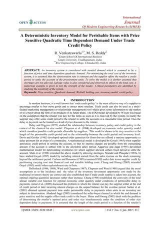
6. A Deterministic Inventory Model for Perishable Items with Price Sensitive...
| IJMER | ISSN: 2249–6645 | www.ijmer.com | Vol. 7 | Iss. 1 | Jan. 2017 | 28 |
3.2.2. Sensitivity Analysis
We now study sensitivity of the models developed to examine the implications of underestimating and
overestimating the parameters individually and all together on optimal value of total profit. The Sensitive
analysis is performed by changing each of the parameter by -30%, -15%, +15% and +30% taking one
parameter at a time and keeping the remaining parameters are unchanged and finally all parameters are
considered. Since both the models show similar results, we will present only the sensitivity for accelerated
growth model. The results are shown in Table-2. The following observations are made from this table:
(i) The total cost TC (T,p) of the system increases (decreases) with an increase (decrease) in the values of the
parameters a, θ, γand Ic while it decreases (increases) with increase (decrease) in the values of the
parameters b, c, Ieand η.
(ii) However, the total cost TC (T,p) is highly sensitive to the changes in the values of the parameters a , ηand
Ic, moderately sensitive to the changes in θ and slightly sensitive to the changes in the values of the
parameters b, c, Ie, and γ.
(iii) As expected, the increase (decrease) in the variable holding cost decreases (increases) in the value of the
total cost TC (T,p) of the system.
(iv) Similarly the increase (decrease) in the salvage value increases (decrease) the profit of the system.
The variations of TC (T,p) with respect to the values of some important parameters and t1 and t2 are shown in
Fig-4, Fig.-5 and Fig.-6 respectively.
IV. CONCLUSIONS
EOQ models are developed for perishable items with trended demand rate under trade credit policy.
The optimal policies are discussed when the credit period is more than (or less than) the cycle time. When
comparing the two credit periods, it is observed that the total cost of the system is more in case of M  T as
compared with M > T. It is further observed that in both cases the total cost is highly sensitive to the changes in
the mark up price η.
Table-1: a >0, b> 0 and c> 0 (i.e., accelerated growth model)
S.NO. Parameter
%
Change
Change in
T (%)
Change in
p (%)
Change in
TC1 (T, p)
(%)
Change in
Q (%)
1 a
15% -6.1977 -15.8478 14.8440 15.0000
5% -2.1776 -6.0262 4.9480 5.0001
-5% 2.5126 7.0008 -4.9480 -5.0001
-15% 8.0402 25.0972 -14.8440 -15.0000
2 b
15% - - 2.6378 1.0463
5% -3.3501 -37.2212 0.8793 0.3487
-5% 2.1776 37.9051 -0.8792 -0.3487
-15% 5.1926 117.0191 -2.6378 -1.0463
3 c
15% 0.0000 -0.3398 -0.0196 0.0015
5% 0.0000 -0.1118 -0.0065 0.0006
-5% 0.0000 0.1118 0.0066 -0.0006
-15% 0.0000 0.3398 0.0196 -0.0018
4 
15% 1.3400 28.4099 3.3503 0.2255
5% 0.5025 9.4238 1.1167 0.0752
-5% -0.6700 -9.3880 -1.1167 -0.0752
-15% -2.0101 -28.0522 -3.3502 -0.2255
5 Ic
15% 0.0000 0.2101 10.0578 0.0000
5% 0.0000 0.0760 3.3526 0.0000
-5% 0.0000 -0.0849 -3.3526 0.0000
-15% -0.1675 -0.2861 -10.0578 0.0000
6 Ie
15% -8.2077 -30.6764 -0.1414 0.0000
5% -2.6801 -11.4712 -0.0471 0.0000
-5% 2.5126 13.0404 0.0471 0.0000
-15% 7.5377 45.3172 0.1414 0.0000
7 
15% 0.6700 10.5146 0.4357 0.0000
5% 0.1675 3.5049 0.1452 0.0000
-5% -0.1675 -3.5004 -0.1452 0.0000
-15% -0.6700 -10.4967 -0.4357 0.0000
8 
15% 10.0503 -42.4337 -35.6598 -36.0346
5% 2.5126 -27.3638 -13.6942 -13.8383
-5% -2.3451 97.6441 15.8936 16.0605
-15% -29.4807 - 55.7485 56.3344

7. A Deterministic Inventory Model for Perishable Items with Price Sensitive...
| IJMER | ISSN: 2249–6645 | www.ijmer.com | Vol. 7 | Iss. 1 | Jan. 2017 | 29 |
Fig-1: Variations of TC (T,p) w.r.t the values of some important parameters
Fig-2: Variations of Purchase Quantity w.r.t the values of some important parameters
Fig- 3 Variations of Price w.r.t the values of some important parameters
-60
-40
-20
0
20
40
60
80
-20% -15% -10% -5% 0% 5% 10% 15% 20%
TotalCost
% Changes in Parameters
Sensitivity analysis for Total Cost
a=10000
θ=0.05
γ=0.1
I.c=0.16
b=0.25
η=1.1
Pc=8
-60
-40
-20
0
20
40
60
80
-20% -10% 0% 10% 20%
PurchaseQuantity
% Changes in Parameters
Sensitivity analysis for Purchase Quantity
a=10000
I.e=0.12
η=1.1
b=0.25
-40
-20
0
20
40
60
-20% -10% 0% 10% 20%
Price
% Changes in Parameters
Sensitivity analysis for Price
a=10000
θ=0.05
γ=0.1
c=0.001
Ie=0.12
9 Pc
15% - - -3.9216 0.0000
5% -2.5126 -31.4900 -1.3072 0.0000
-5% 1.6750 31.6375 1.3072 0.0000
-15% 3.8526 95.8693 3.9217 0.0000

8. A Deterministic Inventory Model for Perishable Items with Price Sensitive...
| IJMER | ISSN: 2249–6645 | www.ijmer.com | Vol. 7 | Iss. 1 | Jan. 2017 | 30 |
Table-2: a >0, b> 0 and c> 0 (i.e., accelerated growth model)
Fig-4: Variations of TC (T,p) w.r.t the values of some important parameters
Fig-5: Variations of Purchase Quantity w.r.t the values of some important parameters
-50
0
50
100
-20% -10% 0% 10% 20%
TotalCost
% Chanegs in Parameters
Sensitivity analysis for Total cost
a=10000
θ=0.05
b=0.25
I.e=0.12
γ=0.1
-50
0
50
100
-20% -15% -10% -5% 0% 5% 10% 15% 20%
PurchaseQuantity
% Chanegs in Parameters
Sensitivity analysis for Purchase Quantity
a=1000
η=1.1
θ=0.05
b=0.25
S.NO. Parameter
%
Change
Change in
T (%)
Change in
p (%)
Change in
TC2(T, p) (%)
Change in
Q (%)
1 a
15% -7.5503 -19.1849 14.8450 15.0001
5% -2.6846 -7.2902 4.9483 5.0001
-5% 3.0201 8.4604 -4.9483 -5.0001
-15% 9.5638 30.3264 -14.8449 -15.0001
2 b
15% - - 4.3365 1.0446
5% -4.0268 -38.7599 1.4455 0.3481
-5% 2.6846 39.5310 -1.4455 -0.3481
-15% 6.3758 122.6731 -4.3365 -1.0446
3 c
15% 0.0000 -0.3497 0.0379 0.0015
5% 0.0000 -0.1166 0.0126 0.0006
-5% 0.0000 0.1121 -0.0126 -0.0006
-15% 0.0000 0.3452 -0.0378 -0.0018
4 
15% 1.8456 29.4118 2.7717 0.2253
5% 0.6711 9.7471 0.9239 0.0750
-5% -0.6711 -9.7113 -0.9239 -0.0750
-15% -2.3490 -29.0127 -2.7717 -0.2253
5 Ie
15% -8.3893 -31.1603 9.9489 0.0000
5% -3.0201 -12.3655 3.3163 0.0000
-5% 3.3557 15.1228 -3.3163 0.0000
-15% 10.5705 57.6220 -9.9488 0.0000
6 
15% 0.8389 10.9084 0.4330 0.0000
5% 0.3356 3.6316 0.1443 0.0000
-5% -0.1678 -3.6361 -0.1443 0.0000
-15% -0.8389 -10.8949 -0.4329 0.0000
7 
15% 13.0872 -37.8094 -35.6621 -36.0346
5% 3.1879 -26.2554 -13.6951 -13.8381
-5% -2.8523 95.0771 15.8946 16.0607
-15% -38.0872 - 55.7523 56.3345
8 Pc
15% - - -3.8966 0.0000
5% -3.0201 -32.6982 -1.2989 0.0000
-5% 2.0134 32.8237 1.2989 0.0000
-15% 4.6980 99.5606 3.8966 0.0000

9. A Deterministic Inventory Model for Perishable Items with Price Sensitive...
| IJMER | ISSN: 2249–6645 | www.ijmer.com | Vol. 7 | Iss. 1 | Jan. 2017 | 31 |
Fig- 6: Variations of Price w.r.t the values of some important parameters
REFERENCES
[1]. Halley, C.G. and Higgins, R.C., Inventory Policy and Trade Credit Financing, Management Science, Vol. (20),
464 – 471, (1973).
[2]. Chapman, C. B., Ward, S. C., Cooper, D. F. & Page, M. J., Credit Policy and Inventory Control, Journal of the
Operational Research Society, Vol. (35), 1055 – 1065, (1984).
[3]. Davis, R.A. and Gaither, N., Optimal Ordering Policies Under Conditions of Extended Payment Privileges,
Management Sciences, Vol. (31), 499-509, (1985).
[4]. Goyal, S.K., Economic Order Quantity under Conditions of Permissible Delay in Payment, Journal of the
Operational Research Society, Vol. (36), 335–338, (1985).
[5]. Dallenbach, H.G., Inventory Control and Trade Credit, Journal of the Operational Research Society, Vol. 37, 525 –
528, (1986).
[6]. Ward, S.C. and Chapman, C.B., Inventory Control and Trade Credit –A Reply to Dallenbach, Journal of
Operational the Research Society, Vol. 32, 1081 – 1084, (1987).
[7]. Chapman, C.B. & Ward, S.C., Inventory Control and Trade Credit –A Future Reply, Journal Of Operational
Research Society, Vol. 39, 219 – 220, (1988).
[8]. Dallenbach, H.G., Inventory Control and Trade Credit – A Rejoinder, Journal of the Operational Research Society,
Vol. 39, 218 – 219, (1988).
[9]. Shah, V.R., Patel, H.C. and Shah. Y.K., Economic Ordering Quantity when Delay in Payments of Orders and
Shortages are Permitted, Gujarat Statistical Review, Vol. (15), 51 – 56, (1988).
[10]. Carlson, M.L. and Rousseau, J.J., EOQ under Date-Terms Supplier Credit, Journal of the Operational Research
Society, Vol. 40 (5), 451–460, (1989).
[11]. Mandal, B.N. and Phaujdar, S., Some EOQ Models under Permissible Delay in Payments, International Journal of
Managements Science, Vol. 5(2), 99–108, (1989a).
[12]. Mandal, B.N. &Phaujdar, S., An Inventory Model for Deteriorating Items and Stock Dependent Consumption
Rate, Journal of Operational Research Society, Vol. (40), 483–488, (1989b).
[13]. Aggarwal, S.P. and Jaggi, C.K., Ordering Policies of Deteriorating Items under Permissible Delay in Payments, J.
Oper. Res. Soc., Vol. 46(5), 658–662, (1995).
[14]. Chung, K.J., A Theorem on the Deterioration of Economic Order Quantity under Conditions of Permissible Delay
in Payments, Computers and Operations Research, Vol. 25, 49 – 52, (1998).
[15]. Jamal, A. M. M., Sarker, B. R.& Wang, S., Optimal Payment Time for a Retailer under Permitted Delay of
Payment by the Wholesaler, International Journal of Production Economics, Vol. 66, 59 – 66, (2000).
[16]. Sarker, B. R., Jamal, A.M.M. and Wang, S., Optimal Payment Time under Permissible Delay for Production with
Deterioration, Production Planning and Control, Vol. 11, 380 – 390, (2001).
[17]. Abad, P.L. &Jaggi, C.K., A Joint Approach for Setting Unit Price and the Length of the Credit Period for a Seller
when End Demand is Price Sensitive, International Journal of Production Economics, Vol. 83 (2), 115–122,
(2003).
[18]. Chung, K.J. & Huang, Y.F., The Optimal Cycle Time for EPQ Inventory Model under Permissible Delay in
Payments, International Journal of Production Economics, Vol. 84 (3), 307–318, (2003).
[19]. Shinn, S.W. & Hwang, H., Retailer’s Pricing and Lot – Sizing Policy for Exponentially Deteriorating Products
under the Conditions of Permissible Delay in Payments, Computers and Industrial Engineering, Vol. 24(6), 539 –
547, (2003).
[20]. Chung, K.J., Goyal, S.K. & Huang, Yung-Fu, The Optimal Inventory Policies under Permissible Delay in
Payments Depending on the Ordering Quantity, International Journal of Production Economics, Vol. 95(2), 203–
213, (2005).
[21]. Huang, Y.F., Optimal Retailer’s Replenishment Decisions in the EPQ Model under Two Levels of Trade Credit
Policy, European Journal of Operational Research, Vol. 176 (2), 911–924, (2007).
[22]. Teng, J.T., Chang, C.T., Chern, M.S.,& Chan, Y.L., Retailer’s Optimal Ordering Policies with Trade Credit
Financing, International Journal of System Science, Vol. 38 (3), 269–278, (2007).
-50
0
50
100
-20% -15% -10% -5% 0% 5% 10% 15% 20%
Price
% Chanegs in Parameters
Sensitivity analysis for Price
a=10000
θ=0.05
c=0.001
I.e=0.12
γ=0.1