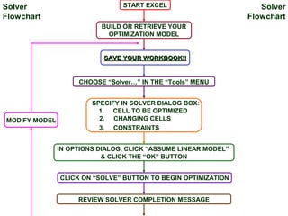
1. Solver START EXCEL Solver
Flowchart Flowchart
BUILD OR RETRIEVE YOUR
OPTIMIZATION MODEL
SAVE YOUR WORKBOOK!!
CHOOSE “Solver…” IN THE “Tools” MENU
SPECIFY IN SOLVER DIALOG BOX:
1. CELL TO BE OPTIMIZED
MODIFY MODEL 2. CHANGING CELLS
3. CONSTRAINTS
IN OPTIONS DIALOG, CLICK “ASSUME LINEAR MODEL”
& CLICK THE “OK” BUTTON
CLICK ON “SOLVE” BUTTON TO BEGIN OPTIMIZATION
REVIEW SOLVER COMPLETION MESSAGE

2. NO SOLVER FOUND
OPTIMUM SOLUTION?
YES
CLICK “KEEP SOLVER SOLUTION”
& CLICK “OK” BUTTON
YES WANT TO CHANGE MODEL
AND RE-OPTIMIZE?
NO
SAVE FINAL MODEL AND
EXIT EXCEL

3. Overview of Solver
LP Modeling Terminology Solver Terminology
Objective function Set Cell
Decision variables Changing Variable Cells
Constraints Constraints
Constraint functions (LHS) Constraint Cell Reference
RHS Constraint or Bound
LP Model Assume Linear Model or
Standard Simplex LP
NOTE: if you get a negative decision and it is not meaningful
to your model, be sure to specify the nonnegativity
constraints in your LP model before optimizing with Solver.

4. The Solver Parameters dialog box will appear.
By default, Max is selected (for maximization) and the cursor
is in the first edit field: Set Target Cell.
Look for the Premium button. If it is not there, then you have
not installed Premium Solver for Education (available from
the CD). Please install this version.

5. Clicking on Premium allows you to specify the type of
optimization that it will perform.
We will use the default Standard Simplex LP
optimization.

6. With your cursor in the Set Target Cell: edit field, specify
the cell to be optimized (i.e., your model’s performance
measure).
The easiest way to do this is to move the dialog (drag
the title bar) so that cell D4 is exposed and then click on
that cell.
You can also click on the button in the edit field
of the dialog to collapse the dialog, click on the cell, and
then click on the button to expand the dialog.

7. The Equal to: field allows you to specify the type of
optimization. You can either maximize or minimize the
performance variable or cause the Target Cell to be
equal to a value of your choosing (select Value of:).
Specify the Oak Product model’s decision variables
(cells B4:C4) in the By Changing Cells: edit field.

8. To specify the constraints, click on the Add button to
open the Add Constraint dialog.
For the LHS of the
constraint, specify
the cell ranges for
the Total LHS of
either one
constraint or a
group of similar
constraints (i.e.,
constraints with the
same inequality) in
the Cell Reference:
edit field of the Add
Constraint dialog.

9. For the RHS of the constraint, specify the cell ranges of
either one resource limitation or a group of similar
limitations in the Constraint: edit field.
Note that when
specifying many
constraints at the
same time, the
number of cells
referenced in the
LHS must equal
the number in the
RHS.
Click Add to add these constraints to Solver.

10. Finally, add the
Chair Production
constraint.
Note that the
inequality is > for
this constraint.

11. Here is the resulting Solver dialog after adding all of the
constraints:
Now, in the Solver Parameters dialog, click the Options
button to specify a linear model.

12. In the resulting Solver Options dialog, click on the
following options:
Assume Linear Model
(Specifies an LP
model, same as
Standard Simplex
LP)
Assume Non-Negative
(Apply nonnegativity
constraints)
Use Automatic Scaling
(to be discussed later)

13. Click OK to return to the Solver Parameters window and
then click Solve to start the optimization.
Remember that this is an iterative technique and may
take a few seconds or a few minutes depending on the
size of the model.
When completed, the Solver Results dialog will appear.
It is important to check to see if Solver found a solution and
if all constraints and optimality conditions were satisfied.
This information will be displayed in the first sentence in this
dialog. ALWAYS READ THIS SENTENCE!

14. Upon the successful completion of the Solver program,
you have the following options:
Keep the Solver Solution
Restore the Original Values (throw the solution away)
Receive up to three reports on the solution (each
formatted as a new worksheet added to the Excel
workbook.
NOTE: The Premium edition may also list an Infeasibility
Report and a Non-Linear Report if there is a problem.

15. Recommendations for Solver
Three LP modeling habits you should develop for better
use of Solver:
1. Make sure the numbers in your LP model are
scaled such that the difference between the
smallest and largest numbers in the spreadsheet
is no more than 6 or 7 digits of precision (e.g., .05
and 10.00 is an acceptable range while .05 and
1,000,000 is not).

16. Recommendations for Solver
2. All RHS’s in the Constraints section of the Solver
Parameters dialog should contain cell references
(to the RHS cells in the spreadsheet model itself),
and
The RHS cells on the spreadsheet model itself
should contain constants and not formulas (or
more precisely, no formulas that involve decision
variables directly or indirectly).

17. Recommendations for Solver
3. Use Excel’s Range Naming commands to give
range names to the performance measure cell, its
decision cells, its constraint function (Total LHS)
cells, and its RHS cells.
These names will automatically be substituted for
the corresponding cell ranges in the Solver
Parameters dialog.