Uncertainty in simulating biomass yield and carbon-water fluxes from Euro-Med...
AGU_2014 Poster_v3
1. Objective: To evaluate the ability of the CRDS method to measure CO2, CH4,
and N2O fluxes from saltmarshes by:
1. Comparing CO2, CH4, and N2O fluxes measured using the Shimadzu
Gas Chromatograph 2014 (GC) and CRDS Picarro G2508 Analyzer.
2. Comparing N2O fluxes measured using the CRDS Picarro G2508 Analyzer
and Los Gatos N2O/CO analyzer (LGR) – a mid-IR spectrometer.
Using Near-IR Cavity Ring-Down Spectrometry to Simultaneously Measure N2O, CO2, and CH4 Fluxes:
Responses to Ammonium Nitrate Additions in Salt Marshes
Elizabeth Brannon1, Serena Moseman-Valtierra1, Jianwu Tang2, Xuechu Chen2, Rose Martin1, Melanie Garate1
1University of Rhode Island Department of Biological Sciences, 2Marine Biological Laboratory Ecosystems Center
Introduction
• Salt marshes are known to
sequester carbon but may also be
sources of three greenhouse
gases (GHGs): CO2, CH4, and
N2O1-12.
• Factors that impact the magnitude
of GHG fluxes from salt marshes
include temperature, plant and
animal species present, above
ground biomass, nutrient input,
flood stage, soil composition, light,
and salinity2, 3, 5, 6, 8-10, 12, 13.
• Due to the complexity and
variability of the system especially
in the face of climate change,
need continuous data on GHG
fluxes.
• Development of cavity ring down
spectroscopy (CRDS) as a tool
to measure GHGs has potential to
fill this data gap.
• In the Picarro G2508 analyzer
(Picarro), CRDS uses infrared
lasers to measure CO2, CH4, and
N2O simultaneously every second.
Figure 1. Saltmarshes sequester a lot of
carbon but more data is needed on whether
CO2, CH4, and N2O may offset this
sequestration.
Figure 2. Diagram demonstrating CRDS14.
General Methods
• For lab analyses, live plants and sediments were collected from RI salt
marshes
• Objective 1: CO2, CH4, and N2O concentrations measured from samples
simultaneously with Picarro and GC samples (Figure 3).
• Objective 2: N2O concentrations were measured simultaneously with
Picarro and LGR in the lab and field (Figure 4).
Literature Cited:
1. Allen et al. (2007). Soil Biology and Biochemistry, 39, 622-631.
2. Bartlett et al. (1985). Journal of Geophysical Research, 90 (D3), 5710-5720.
3. Bartlett et al. (1987). Biogeochemistry, 4, 183-202.
4. Chmura et al. (2003). Global Biogeochemical Cycles, 17 (4), 22-1 to 22-12.
5. DeLaune et al. (1983). Tellus, 35B, 8-15.
6. Giani et al. (1996). European Journal of Soil Science, 47, 175-182.
7. McLeod et al. (2011). Ecological Society of America, 9 (10), 552-560.
8. Hirota et al. (2007). Chemosphere 68, 597-603.
9. Liikanen et al. (2009). Boreal Environment Research, 14, 351-368.
10. Magenheimer et al. (1996). Estuaries, 19 (1), 139-145.
11. Mortazavi et al. (2012). American Geophysical Union, Fall Meeting 2012, abstract #B51B-0549.
12. Tong et al. (2010). Journal of Environmental Science and Health, Part A: Toxic/Hazardous Substances and Environmental Engineering, 45 (4), 506-516.
13. Moore et al. (1994). Journal of Geophysical Research, 99 (D1), 1455-1467.
14. http://www.picarro.com/technology/cavity_ring_down_spectroscopy
Sample
Type
Trial
#
Picarro GC Paired
T-test
p-value
Paired
T-test
DFR2 Flux
(µmol m-2
h-1
)
Flux
(µmol m-2
h-1
)
R2
Sediment
Only
1 0.513 ND 0.0 0.002
NA NA2 0.023 ND 0.0 0.007
3 0.275 ND 0.0 0.015
Phragmites
4 0.974 4663.9 4424.7 0.932
0.076 25 0.997 1361.6 943.1 0.808
6 0.998 1017.3 866.8 0.747
Objective 1: Picarro/GC Comparisons
Table 1. CH4 results of Picarro/GC comparison. Bolded R2 indicates the
regression had a significant p-value.
Results:
• The Picarro was able to detect lower N2O, CH4 , and CO2 and fluxes than
the GC (Figure 6A, Tables 1 and 2).
• Fluxes that were measured with the Picarro had consistently greater R2
values than those from a GC (Figures 5 and 6B, Tables 1 and 2).
CH4: When a flux was detected by the GC, there was no significant
difference between the flux measured by the GC and Picarro (Table 1).
Sample Type
Trial
#
Picarro GC
R2 Flux
(µmol m-2
h-1
)
Flux
(µmol m-2
h-1
)
R2
Sediment
Only
1 0.987 6452.9 0.0 0.005
2 0.988 5456.8 0.0 0.110
3 0.970 4632.2 0.0 0.198
Phragmites
6 0.995 113979.8 ND 0.526
7 0.999 69711.7 0.0 0.102
8 0.999 58918.5 0.0 0.215
Table 2. CO2 results of Picarro/GC comparison. Bolded R2 indicates the regression
had a significant p-value.
CO2: The GC was not able to detect any CO2 fluxes. Therefore no statistics
were performed (Table 2).
Objective 2: Picarro/LGR Comparison-Lab
Acknowledgments: Funding for this project is provided by the USDA
RI Hatch Grant #4002, NOAA/National Estuarine Research Reserve
System Science Collaborative and NOAA Sea Grant. I would like to
thank Isabella China and Kate Morkeski for help in the field. I would
also like to thank Inke in the Lars Kutzbach lab for the Matlab script
used to calculate fluxes.
Conclusions
1. Picarro analyzer is able to detect lower CO2, CH4, N2O fluxes than the GC.
2. N2O fluxes >150 umol m-2 hr-1 measured by the Picarro and LGR are
comparable.
3. These experiments suggest that near-IR CRDS technology offers a new tool for
simultaneous analyses of N2O along with CO2 and CH4, which fills an important
need for quantifying the net climatic forcing of ecosystems.
4. Based on relatively high minimum N2O detection levels of the CRDS
(5 µmol m-2 hr-1), it may work best in highly eutrophic environments.
• Flux calculation performed in Matlab: Flux=dC/dt(PV/RAT)
• dC/dt = Change in concentration over the time the chamber was deployed
• P = pressure
• V = volume of chamber
• R = gas constant
• A = area covered by chamber
• T = temperature determined by Hobo logger (Onset Inc.)
• Data Criteria:
• If R2>0.70 and p-value <0.05 = Significant flux
• If R2<0.70 but p-value <0.05 = Non Detectable (ND)
• If R2<0.70 and p-value >0.05 = Zero flux
• For some Picarro and LGR data a 15 second average was used
• Statistics were performed in JMP 11, Excel, and Matlab
• Regression for each chamber (time vs. concentration)
• Paired t-test (Picarro vs. GC or Picarro vs. LGR)
Figure 4. Set up for lab measurements for
Objective 2: Picarro vs. LGR.
Figure 3. Set up for measurements for
Objective 1: Picarro vs. GC.
N2O: When a flux was detected by the GC there was no significant difference
between the flux measured by the GC and Picarro
(t2=0.9314, p-value =0.450).
0
100
200
300
400
500
1 2 3 4 5 6
Trial #
Picarro
GC
N2OFlux
(µmolm-2hr-1)
0 0 0
A
0.0
0.2
0.4
0.6
0.8
1.0
1 2 3 4 5 6
R2
Trial #
B
Figure 6. (A) N2O flux for each trial measured by the Picarro and GC. (B) R2 for each N2O flux for each trial.
Methods:
• Two samples: One with sediment only (Trials 1-3) and one with live
Phragmites (Trials 5-6).
• A series of three chamber deployments were made for each sample
Objective 2: Picarro/LGR Comparison-Lab
Results:
• A wide range of large (Figure 7 A+B) and small fluxes (Figure 7 C+D)
were observed and were analyzed separately.
• For large fluxes there were no significant differences between the Picarro
and LGR (Figure 7 A+B).
• For small fluxes there were significant differences between the Picarro
and LGR (Figure 7 C+D).
• On average N2O fluxes that were measured with the Picarro G2508 were
greater than those measured by the LGR (Figure 7).
Methods:
• Two trials: one with live vegetation and one with sediment only.
• For both trials there was single NH4NO3 addition followed by time series of
N2O measurements.
Figure 7. N2O Fluxes over time for both the LGR and Picarro for (A) Live vegetation high fluxes (B) Sediment
only high fluxes (C) Live vegetation low fluxes (2 points not shown because they were measured several days
later) (D) Sediment only low fluxes.
Low Fluxes: Significant differences between LGR and Picarro for both
trials (t10=4.5249, p-value=0.0011 and t6=4.75, p-value=0.003).
High Fluxes: No significant differences between LGR and Picarro for both
trials (t8=1.7507, p-value=0.1181 and t3=1.8070, p-value=0.1685).
Objective 2: Picarro/LGR Comparison-In-Situ Measurements
Methods
• Location: Sage Lot Pond, Waquoit
Bay, MA
• Two sets of three plots with each trio
receiving different levels of NH4NO3
enrichment (Figure 8).
• Measured N2O concentrations
simultaneously with Picarro and LGR
for 10 minutes from each plot 1 hour
after NH4NO3 additions (Figure 9).
Figure 8. Set up of plots in salt marsh at
Sage Lot Pond, Waquoit Bay, MA.
Figure 9. Chamber deployed in marsh.
Results and Discussion
• N2O fluxes measured with the Picarro
and LGR were significantly different
(t10=2.62, p-value=0.026) (Figure 10)
• On average the Picarro flux was about
10% greater than the LGR flux
(Figure 10).
Figure 10. Percent difference between the Picarro and LGR for each plot and each day of measurements.
y = 0.0019x + 0.461
R² = 0.9684
0.0
0.4
0.8
1.2
0 100 200 300 400
N2O
(ppm)
Seconds
y = 0.0015x + 0.5951
R² = 0.7098
0
0.4
0.8
1.2
0 100 200 300 400
N2O
(ppm)
Seconds
Figure 5. Example N2O data from (A) Picarro and (B) GC.
A B
200
300
400
44 46 48 50
Time Since N Addition (Hours)
N2OFlux
µmolm-2hr-1
70
75
80
85
90
44 45 46 47
(Time Since N Addition (Hours)
B
0
5
10
15
0.00 1.00 2.00 3.00
Time Since N Addition (Hours)
D
0
40
80
120
0 0.5 1 1.5 2 2.5
Time Since N Addition (Hours)
C
N2OFlux
µmolm-2hr-1
A
N2OFlux
µmolm-2hr-1N2OFlux
µmolm-2hr-1
-10%
0%
10%
20%
30%
1A 1B 1C 2A 2B 2C
PercentDifference
betweenPicarroandLGR
Plot ID
Day 1
Day 2
Spartina alterniflora