SlideShare a Scribd company logo
1 of 40
Download to read offline
Page 1 of 40
How to Apply VECM to Detect the J-Curve in the Case of Japan
Kelly Yiyu Lin* and Wenti Du**
*BMO Financial Group, U.S.A. **Akita International University, Japan
Abstract
Japan has been in economic stagnation for more than two decades. The Japanese yen had a substantial
depreciation from 80 yen/U.S. dollar in 2012 to 120 yen/U.S. dollar in 2014. From the third quarter in 2012 to
the third quarter in 2014, Japan’s trade balance deteriorated. In this paper, we applied VECM (vector error
correction model) to detect if the J-curve effect exists in the case of Japan. Results confirm the existence of the
J-curve when the U.S. federal funds rate, as one of the driving forces, affects Japan’s trade balance, as well as its
exchange rate simultaneously.
JEL Codes: B22, B23, B27 ,C53, F14, F47
Keywords: J-Curve, Depreciation, Trade Balance, VECM, Transitional Dynamics
Page 2 of 40
I. Introduction
Japan has been in an economic stagnation for more than two decades. As an attempt to bring the
country out of recession, Prime Minister Shinzo Abe announced his well-known ‘Abenomics’ after his
victory in the 2012 re-election. As a result, the Japanese yen had a substantial depreciation from 80
yen/U.S. dollar in 2012 to 120 yen/U.S. dollar in 2014. Depreciation of the Japanese yen was supposed
to help strengthen Japan’s trade balance as ‘Made in Japan’ would be more competitive in terms of
price in the international markets. However, Japan’s trade balance did not increase as quickly as
expected. Instead, from the third quarter in 2012 to the third quarter in 2014, Japan’s trade balance
deteriorated. This phenomenon is consistent with the early stage of the well-known ‘J-curve’ effect,
where a country’s trade balance worsens following a depreciation of its currency before it begins to
increase. Are we going to observe the J-curve effect in the case of Japan? This paper applies the VECM
(vector error correction model) methodology to investigate whether, and under which circumstances,
the J-curve effect will occur in Japan.
In the early stages following a depreciation of its currency, a country’s terms of trade will deteriorate as
the price of its exports decreases while the price of its imports increases. However, in the longer term, a
country’s exports become more competitive, both in domestic as well as in international markets.
Therefore both domestic and foreign demands increase. As a result, the country’s trade balance
strengthens and reaches a better status than it was before the currency depreciation. However, Rose
and Yellen (1988) applied monthly bilateral as well as aggregate U.S. trade data, from 1960 to 1985, to
an OLS (ordinary least square) model and found that empirical results showed little or no support for a J-
curve effect. They concluded that various assumptions existed for the J-curve effect, such as a demand
that imports must be priced inelastic in the short run, import prices must be elastic to the exchange rate
in the short run, and the export value must respond slowly to the exchange rate.
In addition, Bahmani-Oskooee and Ratha (2004) reviewed several existing studies that analyzed the J-
curve effect. They concluded that regardless of whether or not bilateral or aggregate data was used with
any type of model, results showed that the short-run reactions of the trade balance on depreciation did
not have a specific pattern. In other words, there was not a consensus on the existence of the J-curve
effect.
Focusing on the case of Japan, Bahmani-Oskooee and Goswami (2003) used quarterly bilateral and
aggregate trade data, from 1973 to 1998, to determine if there was a J-curve effect between Japan and
Page 3 of 40
its nine major trading partners (Australia, Canada, France, Germany, Italy, Netherlands, Switzerland, the
U.K., and the United States). Even though no such effect was found when using aggregate data, the
authors concluded that when they applied bilateral trade data, they found evidence of the J-curve effect
between Japan and Germany and Japan and Italy. In addition, results suggested that the yen’s real
depreciation had positive long run effects in the cases of trade between Japan and Canada, the U.K. and
the United States.
Furthermore, Shimizu and Sato (2015) explained the limited impact of the yen’s depreciation on the
country’s trade balance in the short run by using an auto-regressive distributed lag (ARDL) model in the
time period between January 1985 and June 2014. They concluded that the strategic relocation of
production adopted by Japanese companies, which was to increase overseas production of low-end
products and to focus domestic production on high-end products, was one of the main causes that led
to ineffectiveness of the yen’s depreciation in improving Japan’s trade balance. Moreover, the authors
argued that even though the yen depreciated, agreed upon export prices in contracts were constant,
which was another main reason explaining the deterioration of Japan’s trade balance following the
depreciation of the yen.
In this paper, we develop an econometric model and use the VECM methodology to analyze whether or
not the J-curve effect exists in the case of Japan. Results not only confirm the existence of the J-curve
effect, but also show that such an effect occurs when the U.S federal funds rate, as one of the driving
forces, affects Japan’s trade balance and exchange rate simultaneously in the transitional dynamics. In
other words, a shock from the U.S federal funds rate affects Japan’s exchange rate and turns it into an
exogenous shock on the country’s trade balance, which brings about the J-curve effect.
II. An Overview of Japanese Economy
Japan, the only developed country in Asia, has been experiencing a recession for more than two
decades. Japan's GDP has been stagnant and there has not been significant production growth for
Japanese industries. In order to stimulate the Japan's economy, the Bank of Japan implemented
monetary expansion policies in the previous years. Bernanke (2000, 2002) indicates that such an
accommodative policy can also induce exchange rate depreciation, which might shift the aggregate
demand through improvement of net exports. Japan's economy has been in a liquidity trap during the
previous two decades, so money and bonds become perfect substitutes (Krugman 1998), and the money
from monetary expansion did not go to the money market fully for business transactions. Thus, the
Page 4 of 40
depreciation of the Japanese yen was not significant. During the Asian financial crisis (1997) and the
global financial crisis (mid 2008), Japan obtained significant capital inflow to support the appreciation of
the yen and to increase the foreign reserves to resist the impacts of both financial crises. The Japanese
yen obtained significant appreciation since September 2008 and hit a post war record high (75.32) in
October 2011.
Figure 2.1 demonstrates the exchange rate of Japan
In the face of significant appreciation of the yen, Japanese firms conducted a strategic relocation of
their production. Japanese firms moved domestic production of low-end goods to overseas subsidiaries
and concentrated their domestic production on high-end products1
. Japanese exports, in terms of the
contract (invoice) currency, have not changed in response to the large rate fluctuations of the yen.
Japanese exporters have a strong intent to pursue a price-to-market (PTM) strategy to overcome the
unprecedented appreciation of the yen, from 2009 to 2012, in order to minimize the loss in their profits.
Because of the price-to-market (PTM) strategy, the export prices measured in contract (invoice)
currency has been relatively stable since 2000, regardless of exchange rate fluctuation. Japan is a
developed country with limited natural resources, and it thus relies significantly on imports. The
appreciation of the yen would help Japanese firms to purchase parts and raw material at better prices in
order to produce high end products for exports. The price-to-market (PTM) strategy helps Japanese
1 Of course, there are other reasons besides the appreciation of the Yen that lead to the relocation of production,
such as the increasing cost of labor in Japan and imposing of trade barriers to Japanese exports.
Page 5 of 40
firms to obtain large foreign exchange gains, and the strategic relocation policy helps Japanese exports
to stay competitive.
Figure 2.2 Demonstrates Japan Foreign Exchange Reserves (1268006 USD Million)
Figure 2.2 demonstrates how Japan foreign exchange reserves increase significantly from 1996 to 2012
and then become stagnant after 2012. This chart indicates significant capital inflows during this period,
and supports the appreciation of the yen from 2008 to 2012. The money supply in Japan is made up of
Japanese foreign exchange reserves and Japanese government bonds. In order to keep a stable money
supply, the Japanese government has to sell government bonds in the face of a significant increase of
foreign reserves for sterilization purposes. They sell bonds for sterilization in the face of capital inflows,
which would make the price of bonds lower and pushes the interest rate up. However, Japan has been
in a liquidity trap for the previous two decades. Money and bonds become perfect substitutes, which
lowers interest rates. Japan should sell new bonds for sterilization purposes, instead, they print more
money to pay for the previous debt so it causes the liquidity trap, which causes a deflation risk for Japan,
but not a risk of inflation in the face of significant capital inflows, the depreciation of the yen from
monetary expansion is not apparent. The growth of Japan foreign exchange reserves become stagnant
after 2012, which means there might have been significant capital outflows after 2012. These significant
capital outflows would cause the depreciation of the yen. The appreciation of the yen from 2008 to
2012 leads to the significant decline of the trade balance of Japan (Figure 2.3). Prime minster of Japan,
Shinzo Abe’s economic stimulus package is intended to depreciate the yen sharply from the end of 2012
to stimulate the economy and improve the trade balance of Japan.
Page 6 of 40
Figure 2.3 Demonstrates the relationship between trade balance of Japan and exchange rate of Japan.
The trade balance of Japan declines after 2011. The foreign exchange reserves stays stagnant after 2012,
so there should be no significant capital inflows to make the yen strong. Abe’s economic stimulus
package hopes to stimulate the Japan's economy and improve its trade balance, which significantly
depreciates the yen from 80 in 2012 to 120 in 2014. However, the trade balance declines, rather than
increase, and the yen depreciate, Therefore, the J-curve phenomena occurs between 2012 Q3 and
2014Q3 (circle in Figure 2.3). From 2014 Q2 to 2015 Q4, Japan's trade balance and the yen depreciation
improve from Abe’s economic stimulus package. Japanese firms conduct a strategic relocation of their
production and a price-to-market (PTM) strategy so the export prices measured in contract (invoice)
currency remain relatively stable since 2000, regardless of the exchange rate fluctuations. Therefore the
export effects of the yen depreciation are mitigated. A weaker yen causes an increase in Japanese
exports, but also induces imports of parts and components produced by Japanese overseas subsidiaries.
Therefore, we could say that the depreciation of the yen would not make Japan's foreign exchange rate
become an exogenous shock in the economy. Japan's foreign exchange rate is one of the endogenous
variables for the trade balance model if there is no other significant driving force to make the foreign
exchange rate become exogenous.
After the Great East Japan Earthquake in March 2011, there was an increase in energy imports due to
the shutdown of nuclear plant that causes a trade deficit for Japan. However, the oil price started to fall
from the mid-2014 and the trade deficits improved. Abe’s economic stimulus package depreciates the
Page 7 of 40
yen sharply from the end of 2012 and does not improve the trade balance in the first two years (2012 to
2014), but the trade balance truly improved from 2015 to 2016. Japanese firms conduct a relocation
policy strategy to produce the low-end products overseas, and high-end products domestically. They
conduct research and development (R&D) activities at the headquarters in Japan. Abe’s economic
stimulus package would make Japanese firms become more inclined to accumulate as much earnings as
possible from overseas assets as an income surplus, if the Japanese government implemented a tax
exemption for foreign income. The Japanese economy should obtain more income effects for recovery
from the income surplus.
Figure 2.4 Demonstrates the relationship between trade balance of Japan and yearly growth of U.S GDP
The significant growth of U.S GDP from 2012Q3 to 2014Q4 (circle in Figure 2.4) causes the strong
expectation of an increase of the U.S. federal funds rate, which should be the exogenous shock to
Japan's foreign exchange rate.
Page 8 of 40
Figure 2.5 Demonstrates the economic interaction between foreign exchange rate of Japan and U.S Fed
Funds rate.
The United States is one of Japan's major trading partners, and the U.S. economy leads the Japanese
economy. Interest rate is the instrument for the exchange rate. The U.S. federal funds rate is the real
U.S. interest rate. The U.S. federal funds rate (interest rate) and Japan's foreign exchange rate are
theoretically related by capital mobility. The U.S. federal funds rate leads the movement of Japan's
foreign exchange rate. When the U.S federal funds rate increases, the yen depreciates. According to the
Mundell-Fleming model, the increase of the U.S federal funds rate would attract more capital inflows to
the United States from other countries including Japan. The impact of Japan's capital outflows would
make the yen depreciate. Figure 2.5 demonstrates the yen depreciating to 120 per dollar when the U.S.
federal funds rate reaches the peak at 5% from 2004 to 2008. When the U.S. federal funds rate stays
low, from 2009 to 2012, the yen appreciates and hits a post war record high of 75.32 per dollar in
October 2011. Abe’s economic stimulus package depreciates the yen sharply from the end of 2012, so
the yen depreciated from 2012 to 2015 with low a U.S. federal funds rate. After 2015, the U.S. economy
had a significant recovery and eliminated the risk of deflation, so the U.S. federal funds rate increases
significantly. According to the base scenario of 2017 CCAR economic analysis, the U.S. federal funds rate
will keep increasing from 2017 to 2019, which would cause the depreciation of the yen. Thus, the U.S.
federal funds rate could be the major driving force that leads the trade balance of Japan.
Page 9 of 40
Figure 2.6 demonstrates Japan's foreign exchange rate and a weighted average of the foreign exchange
value of the U.S. dollar against the currencies of a broad group of major U.S. trading partners (US
TRADEW) are co-integrated.
TRADEW is a weighted average of the foreign exchange value of the U.S. dollar against the currencies of
a broad group of major U.S. trading partners including Japan. The broad currency index includes the
Euro Area, Canada, Japan, Mexico, China, United Kingdom, Taiwan, Korea, Singapore, Hong Kong,
Malaysia, Brazil, Switzerland, Thailand, and the Philippines. Thus, TRADEW and Japan's foreign exchange
rate are co-integrated and have the same movements. If the United States enhances business with its
trading partners, Japan's economy should improve as well as other U.S. major trading partners.
Figure 2.7 demonstrates the relationship between Japan's trade balance and the U.S. industrial
production index (US IPI).
Page 10 of 40
The U.S industrial Production index (U.S IPI) measures the real output produced by the manufacturing,
mining, and electric and gas utilities industries in the United States, so the U.S IPI is considered to be the
real production of the United States, which leads Japan's economy and the economy of other countries
in the world. The U.S. IPI is sensitive to consumer demand and interest rates. Because the U.S. IPI is
sensitive to demand, the U.S. domestic demand should increase along with the growth of the U.S IPI.
The increase of U.S. domestic demand would enhance the trading between the United States and Japan.
Thus, Japan's trade balance should improve. The U.S IPI starts to grow significantly since 2009. The
growth of the U.S. IPI would lead the growth of the Japanese economy and enhanced the trade between
U.S the United States and Japan. The U.S. IPI is the major driving force to lead the world economy.
Japan's trade balance declined from 2012 to 2014 when the yen depreciates sharply due to Abe’s
economic stimulus package.
Figure 2.8 demonstrates the relationship between the U.S. IPI and the U.S. federal funds rate.
The U.S. IPI is sensitive to the U.S. federal funds rate and has the same movements from 2003 and 2008.
The U.S. federal funds rate is considered to be the United States' real interest rate. When the economy
was overheated in 2006 and 2007, the U.S Federal Reserve’s bank had to increase the interest rate to
avoid inflation. Because of the global financial crisis, the U.S. government tried to decrease the interest
rate to stimulate the economy, which makes the U.S. federal funds rate close to zero from 2009 to 2015,
with governmental intervention to stimulate U.S. IPI growth. The U.S. IPI did not grow, but declined with
low interest rates, causing a risk of deflation in 2015. The U.S. Federal Reserve’s bank has to increase the
interest rate to eliminate the risk of deflation in 2016. The base scenarios of the 2017 U.S Federal
Reserve’s bank CCAR economic analysis demonstrates that the U.S Federal Reserve’s bank will continue
Page 11 of 40
to increase the interest rate from 2017 Q1 to 2019 Q4, and the U.S. IPI should grow along with the rising
interest rate.
Figure 2.9 demonstrates the relationship between U.S IPI and U.S BBB Corporate risk spread
U.S. credit spreads tend to widen during recession and to shrink during expansion. The credit spread is
due to credit or default risk. The BBB rated bond is less during good economic times. The U.S. BBB
corporate risk spread could be the measurement of industry risk. The higher the U.S. BBB corporate risk
spread is, the lower U.S. industry production is supposed to be. The U.S. BBB corporate risk spread
reached its peak in the global financial crisis period, so U.S. industry productions touch the trough during
that period. The economic analysis of 2017 CCAR indicates that U.S. industrial production would grow
significantly with the low risk index of the U.S. BBB corporate risk spread.
Page 12 of 40
Figure 2.10 demonstrates the CCAR economic scenarios of GDP of Japan.
Japan has been in a recession for more than twenty years. The scenarios of the 2017 CCAR economic
analysis indicates that Japan's GDP would grow strongly. There are a few reasons to that would make
Japan's GDP obtain significant growth after the end of 2016. For example, the recovery of the U.S.
economy could cause the growth of the Japanese economy, so Japan's GDP would grow. Abe’s economic
stimulus package enhances the trading with the Japan's trading partners after 2015. This stimulus makes
Japanese firms become more inclined to accumulate as much earnings of overseas assets as possible as
income surplus if the Japanese government implemented a tax exemption for foreign income. Japan's
economy would obtain more capital for growth and then obtain significant growth of the GDP. Different
from the stagnant GDP before 2014, the growing GDP of Japan would become the driving force of the
trade balance model.
III Data and Methodology
Quarterly data from Japan’s trade balance, the U.S industrial production index and Japan’s foreign
exchange rate were collected from various sources. The quarterly data from Japan's trade balance came
from the Bank of Japan. The U.S. industrial production index and Japan's foreign exchange rate came
from U.S Federal Reserve's Bank. The data for model specification spans from 2003Q1 to 2016Q3, which
includes the period of the Global Financial Crisis (2008Q3-2010Q4) as well as the period of the recovery
(2011Q4-present). This paper includes the stress testing of Japan's trade balance, where the driving
forces of the Vector Error Correction Model (VECM) came from the U.S. Federal Reserve Bank’s 2017
Page 13 of 40
CCAR. The driving forces are exogenous and the major driving forces for Japan's trade balance are the
U.S federal funds rate, the U.S. BBB corporate risk spread, Japan's GDP and TRADEW (a weighted
average of the foreign exchange value of the U.S. dollar against the currencies of a broad group of major
U.S. trading partners. The data for the economic analysis covers the periods of the Japanese recession in
the 1990s, the Global Financial Crisis and recovery of the economy.
Japan is one of the most developed countries in the world and relies on imports from other developed
countries. Japanese firms implement a strategic relocation of their production and price-to-market
(PTM) strategy to resolve the fluctuation of exchange rate for more than 10 years. Although Abe’s
economic stimulus package depreciates the yen sharply, from 80 in 2012, to 120 in 2014, the
depreciation of the yen might not improve the trade balance significantly in the short run. Japan's trade
balance decreased rather than increased from 2012 to 2014. However, Japan’s trade balance improved
after 2015. As one of Japan's major trading partners, the U.S economy leads Japanese economy. Japan's
economy improved when U.S economy turns better. This paper demonstrates the trade balance model
between the United States and Japan.
The J-Curve phenomena cause currency depreciation, improve the trade balance in the long run, but
worsen the trade balance in the short run. The trade balance model from Rose and Yellen (1989)
indicates that the trade balance is the function of exchange rates and incomes of trade partners. The
trade balance models would be demonstrated as follows:
TB = X·Px - M·Pm = TB (q, Yx, Ym) Equation (3.1)
Where
TB: trade balance of Japan
X: export demand of Japan
Px: price of export
Pm: price of import
M: import demand of Japan
Yx: real income of export country
Ym: real income of import country
q: exchange rate
Page 14 of 40
Equation 3.1 demonstrates the outline of the trade balance model. If we focus on the trade balance
model between the United States and Japan, it would become the function of the exchange rate
(yen/dollar), Japan's industrial production index (JapanIPI), and the U.S. industrial production index
(USIPI). This paper employs the industrial production index to be the real GDP. Since the United States is
one of the major trading partners of Japan, the trade balance between Japan and the United States
should be significantly co-integrated with Japan's total trade balance. Thus, this paper uses Japan's
aggregate trade balance in the trade balance model between Japan and the United States. Because
Japan has been in a recession for more than twenty years, Japan's industrial production index did not
obtain significant growth and remained stagnant during the recession period. Japan's stagnant industrial
production index would cause a collinear problem in the trade balance model, so we have to exclude it..
The revised trade balance model between the United States and Japan should look like Equation (3.2):
JAPANTB = TB (EXJAPAN, USIPI) Equation (3.2)
Equation 3.2 demonstrates the long-run economic interactions of endogenous variables, which includes
the Japan's foreign exchange rate (yen/dollar), and the U.S industrial production index as endogenous
variables. Japan's government is the central planer who tries to maximize the utility of the trade balance
to reach the Pareto optimality condition of the economy. According to the second welfare theorem, the
Pareto optimality of the economy would lead to a competitive equilibrium. Thus, agents would
maximize their utilities; firms would maximize their profits and the market would clear. The Pareto
optimality could be demonstrated in the following mathematic optimization form:
Mathematic optimizations:
MAX {U (USIPI, EXJAPAN)}
s.t. β0 + β1·USIPI + β2·EXJAPAN < = C
£ = U + λ· (C- (β0 + β1·USIPI+ β2·EXJAPAN))
F.O.C:
∇USIPI, EXJAPAN, λ £ (USIPI, EXJAPAN, λ) = 0
Note that ∇ λ £ (USIPI, EXJAPAN, λ) = 0 means β0 + β1·USIPI + β2·EXJAPAN = C
Where
Page 15 of 40
U (JAPANTB): utility of central planner for trade balance
U (JAPANTB) =U (EXJAPAN, USIPI)
JAPANTB: the trade balance of Japan
USIPI: US industrial production index
EXJAPAN: exchange rate of Japan (yen/dollar)
C: constant level of trade balance; C > 0
Milton Friedman said that the best model should be the model that provides the best forecasts. This
should hold when the model achieves the Pareto Optimality. Both the multivariate time-series model
(VECM) and mathematic optimization demonstrates the framework of Pareto Optimality. Specifically,
the multivariate time-series model accommodates the impacts of exogenous shocks and uses the
resources to maximize the utility of the central planner so that the Pareto Optimality is achieved. For the
trade balance model, the central planner is maximizing utility of the central planner subject to the trade
balance constraint of endogenous variables. However, the driving forces (exogenous shocks or
predetermined variables) would lead the model to obtain the best forecasts.
Budget constraint ensures economic interactions of endogenous variables in the steady state (long-run
equilibrium). The first order conditions of the above optimization demonstrate that there is no weakly
exogenous or exogenous condition of endogenous variables in the transitional dynamics (short-run
equilibrium). The exogenous variables are the driving forces, which are the shocks of the model. The
shocks would cause the model to deviate from a steady state. A variable cannot be endogenous and
exogenous variable at the same time. Based on the concept of the mathematic optimization, we specify
the trade balance model in the following steps:
Step 1: We construct an ordinary least square model (OLS) as the baseline model to identify the co-
integration relationship (steady state or long-run equilibrium) of the endogenous variables and specify
the impulse indicators to capture the hit-and-run impacts of the exogenous shocks.
JAPANTB = β0 + β1·EXJAPAN + β2·USIPI + β3·IDUM1 + β4·IDUM2 + β5·IDUM3 + u Equation (3.3)
Where
Page 16 of 40
IDUM1: the impulse indicator captures the uptrend impacts of exogenous shocks
IDUM2: the impulse indicator captures the downtrend impacts of exogenous shocks
IDUM3: the impulse indicator captures the specific outlier impacts of exogenous variables
u: the error terms; the error terms need to be white noise that indicates zero mean, normally
distributed and, no serial correlation of the error term
Equation 3.3 indicates the model is deviating from the steady state when impulse indicators are
significant. The impulse indicators are a type of additive dummies that take a value of “0” or “1.” They
are called “on” or “off” variables, where “1” corresponds to “on”. The impulse indicators capture the
impacts of the exogenous shocks, which ensure the stabilities of parameters and white noise error terms
when the model is deviating from the steady state. The impacts of the exogenous shocks come from the
effects of policy changes, company mergers, regulation changes, and financial crises, etc. The impulse
indicators exclude the non-linear issues from the exogenous shocks. Ignoring the impulse indicators, the
information set would be asymmetric and the model would be incorrectly specified.
JAPANTB = β0 + β1·EXJAPAN + β2·USIPI + є Equation (3.4)
Where refers the error term of the co-integration equation.
Equation 3.4 demonstrates the co-integration relationship (steady state or long-run equilibrium) of
endogenous variables in the trade balance model, which includes Japan's trade balance, foreign
exchange rate and the U.S industrial production index. The definition of co-integration indicates that all
endogenous variables do not have to be stationary, but the first difference of the endogenous variables,
and the linear combination of the endogenous variables (error terms) must be stationary. The OLS
methodology identifies the steady state the model is approaching, and specifies the impulse indicators
needed to capture the hit-and-run impacts of shocks. However, OLS is not able to demonstrate the
economic interactions in the transitional dynamics and judge the driving forces to restore (or deviate)
the model back to the steady state.
This paper is investigating the trade balance model between Japan and the United States. The U.S.
economy leads Japan's economy so the U.S. economic indices should be the driving forces to lead the
trade balance model back to a steady state. It is important to know under what conditions a real
depreciation of the yen improves Japan's trade balance of Japan in the long run, but worsens it in the
Page 17 of 40
short run. Abe’s economic stimulus package depreciates the yen sharply when the Japan's economy is in
a recession. This paper determines if the impacts of the yen depreciation are significant enough to make
Japan's foreign exchange rate cause exogenous shocks in the model, which are the J-curve phenomena.
In order to demonstrate the above economic activities, we apply the multivariate time series model
(VECM) in the step 2.
Step 2: We run the VECM to demonstrate the economic activities in the steady state, and also in the
transitional dynamics. Equation 3.5 demonstrates the VECM.
ΔZ𝑡+1 = C + Σ Гi ΔZ𝑡−𝑖 +αβ’ Z𝑡 + ΦD𝑡 + δΔHt+1 + ε𝑡; i= 1, 2 …...... Equation (3.5)
In the trade balance model of Japan, the lag of VAR is one. Thus, i=1
Zt: the vector of endogenous variables that are JAPANTB (trade balance of Japan), EXJAPAN (foreign
exchange rate of Japan, and USIPI (U.S industrial production index)
β: long run parameter Beta estimates (co-integrating vector)
α: adjustment coefficient Alpha estimation (error correction vector)
β'Zt-1: the vector of co-integrating vector
αβ'Zt-1: the lagged error correction term in VECM
ΔZt: the vector of the first difference of endogenous variables
ΔHt+1: the first difference of risk factors (or predetermined variables); the significant change of risk
factors are exogenous shocks (DJGDP, DTRADEW, DUSBBBCORPRISKSPREAD, and DUSFEDFUNDSRATE)
Dt: Dt includes the impulse indicators (IDUM1 IDUM2 and IDUM3) and driving forces (DJGDP, DTRADEW,
DUSBBBCORPRISKSPREA, and DUSFEDFUNDSRATE)
Єt: the error terms of transitional dynamics of VEC, which need to be white noise
DJGDP: the first difference of GDP of Japan
DTRADEW: the first difference of a weighted average of the foreign exchange value of the U.S. dollar
against the currencies of a broad group of major U.S. trading partners
Page 18 of 40
DUSBBBCORPRISKSPREA: the first difference of U.S corporate risk spread
DUSFEDFUNDSRATE: the first difference of U.S federal funds rate
The Dt of the VECM includes all exogenous factors that are dummy variables (or impulse indicators) and
driving forces (predetermined variables). The exogenous driving forces (shocks) could provide the
impacts to efficiently restore the model back to the steady state when the economy condition is turning
better. The results of Granger causality could provide the candidates of driving forces. It is very
important to identify the economic condition and select the correct driving forces for the VECM. All of
the endogenous variables move simultaneously in the VECM. When we select driving forces, we have to
consider the driving forces for all endogenous variables, not only those for the objective (normalized)
variable in the VECM. All transitional dynamics of endogenous variables of the VECM should exclude the
weakly exogenous. The growth of the U.S economy picks up in 2012Q3 and advances above the 4%
annualized rate for several quarters. The strong recovery of the U.S .economy would cause the strong
expectation of a rise in the U.S federal funds rate. During the recession period, U.S. and Japanese
interest rates are very low and even low enough to cause the risk of deflation. Interest rates are the
instrument for the exchange rate because interest rates and exchange rates are related for capital
mobility. The strong expectation of the increase of the U.S. federal funds rate would affect Japan's
foreign exchange rate as well as its trade balance.
Interest rates could affect the trade balance if international substitution influences consumption and
imports. The U.S. federal funds rate is considered as the real interest rate of the U.S. economy. The
efficient recovery of the U.S. economy would push the rise of the U.S. federal funds rate, which would
cause more capital inflow to the United States from Japan and other countries in the world. The
significant capital inflow would make the U.S. dollar stronger and make the yen weaker. Thus, the U.S.
federal funds rate should be one of the major driving forces of trade balance model between Japan and
the United States. The base scenario of 2017 CCAR economic analysis demonstrates that Japan's GDP
will be no longer stagnant, and grow significantly after 2016 Q3 to 2019Q4. Thus, Japan's GDP should be
the driving force of the trade balance model to mutually improve U.S. and Japanese industrial
production. TRADEW is a weighted average of the foreign exchange value of the U.S. Dollar against the
currencies of a broad group of major U.S. trading partners, including Japan. When the Dollar becomes
strong, TRADEW would become depreciated and enhance the worldwide trading business. Therefore
TRADEW is selected to be one of the driving forces. The U.S. BBB corporate risk spread would affect the
Page 19 of 40
U.S. industrial production index; therefore this is also selected as one of the driving forces for the trade
balance model.
Most of the previous studies used log-level data. However, in order to keep the nature of data, the
baseline OLS model regression is run with data in level without any data transformation. In order to
satisfy the definition of the co-integration, the first difference of endogenous variables and the error
term of co-integration equation have to be stationary. A constant is estimated in OLS and the VECM
models because Japan's trade balance data shows a deterministic drift. Japan's trade balance data
demonstrates certain specific patterns, but not significant enough to be called seasonal patterns. We
incorporate these patterns in the impulse indicators both in-sample and out-of-sample. The forecasts
are based on the historical information set. If the historical information set demonstrates the specific
patterns of data nature, the similar patterns would show up in the future economic activities (forecasts).
Therefore, we have to understand the data nature carefully to specify the impulse indicators both in-
sample and out-of-sample. Under such conditions, we will avoid using too many dummy variables that
would cause the collinear problems. The VECM trade balance model only has one lag. The number of
lags should be less than four (there are four quarters in a year) for a well-specified model if the data of
all endogenous variables are independent and identically distributed random variables.
Most previous papers specify the trade balance model as the following two equations:
The first equation of the model demonstrates the baseline OLS model regression. However, without
imposing any impulse indicators to capture the impacts of exogenous shocks, the model should be miss-
specified and provide the spurious results to demonstrate economic interactions of endogenous
variables. The second equation demonstrates the transitional dynamics by using ARDL (auto-regression
distribution lag) model. However, the second equation makes endogenous variables, except TB, be
exogenous shocks as well. There is no impulse indicator to capture the impacts of exogenous shocks. No
variable can be endogenous and exogenous at the same time in the transitional dynamics. This paper
revises the model and presents better economic intuitions.
Page 20 of 40
IV. Empirical Results
The J-curve phenomena indicate that currency depreciation improves the trade balance in the long-run,
but worsens it in the short run. However, the existence of the J-curve phenomena is in debate. Rose and
Yellen (1989) state no statistically reliable evidence of a stable J-curve is detected when they did
research on the U.S. trade balance model. Rose and Yellen (1989) emphasize that if ordinary least
square (OLS) is used, weak evidence of a J-curve is detected. They also question under what
circumstances a real depreciation improves the real trade balance in the long run and worsen it in the
short run. The J-curve phenomena might occur when there is a certain factor or issue to cause the
exchange rate of trade balance model from endogenous to exogenous, which makes the exchange rate
a significant shock to the trade balance. The most previous studies applied both the OLS and auto-
regressive distribution lag (ARDL) models to demonstrate that the economic activities of the trade
balance model in the long run equilibrium and in the short run dynamics. However, this methodology is
not able to demonstrate the economic activities in transitional dynamics precisely. This paper applied
both the OLS model and the VECM. The OLS model is the baseline model to specify the co-integration
equation and demonstrate the economic activities of endogenous variables in the long run. The VECM
demonstrates that the economic activities in the steady state and in the transitional dynamics. The
results are shown in the followings:
Table 4.1 demonstrates the results of OLS model
Page 21 of 40
Table 4.1 demonstrates high R-square value (0.9517) of the OLS model, which presents the Goodness-of
Fit for the model. The values of VIF (variance inflation) for all variables are less than 3 and the co-
linearity diagnostic index are less than 100, so there are no multi-collinearity and collinear problems in
the model. The multi-collinearity and collinear problems occur because endogenous variables obtain a
certain degree of identical information between each other, which would cause the singular problem of
the model and even make the model break down. All independent variables are significant. The results
of OLS model indicate Japan's trade balance moves positively when the U.S. industrial production index
(USIPI) grows significantly; Japan's trade balance moves gradually when its foreign exchange rate
depreciates significantly.
USIPI and EXJAPAN are endogenous in the model. The depreciation from Abe’s economic stimulus
package would not be strong enough to cause Japan's foreign exchange rate (EXJAPAN) to be
exogenous. The impulse indicators (IDUM1, IDUM2 and IDUM3) are exogenous to capture the impacts
of exogenous shocks, which indicate the model is deviating from the steady state. The function of an
impulse indicator is to stabilize the parameters and capture the hit-and-run impacts in the face of
exogenous shocks. The OLS model helps to define the steady state of trade balance model and to specify
the impulse indicators when the model is deviating from the steady state. The results of applying the
OLS model demonstrates that Japan’s trade balance would move positively and its foreign exchange rate
would depreciate in the long run.
Rose and Yellen (1989) indicate “a J-curve is defined as the combination of a negative short-run
derivative with a positive long-run derivation. The question posed-under what circumstances a real
depreciation improves the real trade balance in the long run but worsen it in the short run --- is distinctly
partial equilibrium in nature”. We apply the VECM to discuss the J-curve in detail after we specify the
baseline OLS models. The results of the VECM are as follows:
Page 22 of 40
Table 4.8 demonstrates the steady state (co-integration equation or the long-run equilibrium) of VECM
We identify the steady state of the trade balance model and test the co-integration (Appendix 1). The
long run equilibrium (co-integration or steady state) of the VECM demonstrates JAPANTB -
65.43019·USIPI – 74.0087·EXJAPAN=0. Because the application of the impulse indicators in the VECM
provide a complete information set, the sign of parameters of independent variables are correct. The
steady state indicates that Japan’s trade balance would increase gradually and its foreign exchange rate
would depreciate while the U.S industrial production index would expand in the long run. The steady
state provides the reliable and stable economic interactions of endogenous variables.
Table 4.9 demonstrates the transitional dynamics of the objective function JAPANTB in the VECM
The objective variable of the trade balance model is JAPANTB, so we normalize JAPANTB in the VECM.
The VECM makes all endogenous variables move simultaneously in response to the exogenous shocks in
the transitional dynamics. We should select the driving forces for all endogenous variables. Driving
forces (predetermined variables) are the exogenous shocks. According to the efficient recovery of U.S
Page 23 of 40
economy, the United States would increase the federal funds rate. However, it is important to
determine if the Federal Reserve’s Bank increases the U.S federal funds rate too much and too fast to
make Japan’s foreign exchange rate become exogenous shock in the trade balance model. The U.S.
federal funds rate and U.S. BBB corporate spread risk are the major driving forces of JAPANTB. The
transitional dynamics of JAPANTB show the shock impacts of the U.S. federal funds rate and U.S. BBB
Corporate risk spread would cause the decline of JAPANTB significantly.
JAPANTB is the objective variable in the trade balance model. We observe that the JAPANTB sustains the
impacts of exogenous shocks in transitional dynamics and that there is no issue with having weakly
exogenous for endogenous variables (USIPI and EXJAPAN) because there is no significant shock impact
of USIPI and EXJAPAN on JAPANTB in the previous period (t-1). The VECM provides the information to
detect when other endogenous variables (EXJAPAN and USIPI) will become exogenous under certain
conditions. When the objective variable (JAPANTB) and other endogenous variables (EXJAPAN and
USIPI) are affected by the same driving force in the VECM simultaneously, the impacts of a driving force
would make that endogenous variable turn exogenous to affect JAPANTB implicitly. This demonstrates
the existence of a J-curve in the trade balance model. This paper will discuss this issue in the following
transitional dynamics.
Table 4.10 demonstrates the transitional dynamics of EXJAPAN in the VECM
The transitional dynamics of EXJAPAN provides the forecast of EXJAPAN and also demonstrates when
EXJAPAN would become exogenous to JAPANTB under certain condition. TRADEW and the U.S. BBB
corporate risk spread are major driving forces for EXJAPAN in the transitional dynamics. The shock
Page 24 of 40
impacts of the U.S. federal funds rate on EXJAPAN are almost significant. There is no weakly exogenous
issue of endogenous variables (JAPANTB and USIPI) on EXJAPAN.
The shock impacts of depreciated TRADEW would cause the depreciation of the yen to compete with
Japan’s trade partners. The shock impact of a rising U.S. BBB corporate risk spread indicates more risk in
the U.S. economy would cause more capital outflows from the United States to Japan and push the yen
appreciated. The shock impacts of a rising U.S .federal funds rate would cause more capital inflows to
the United States from Japan and make the yen depreciated. However, the U.S. federal funds rate is the
driving force that affects JAPANTB and EXJAPAN simultaneously in the transitional dynamics. EXJAPAN
would become exogenous to the trade balance model when the shock impacts of U.S. federal funds rate
affects EXJAPAN significantly, and make EXJAPAN exogenous in the transitional dynamics. Interest rates
are the instrumental variable for the exchange rate. As long as the shock impacts of the U.S. federal
funds rate affect EXJAPAN significantly, EXJAPAN would change from endogenous to exogenous in the
trade balance model implicitly. The following equations demonstrate how the U.S. federal funds rate
would become the driving force to make EXJAPAN become exogenous in the trade balance model.
Equation 4.1 demonstrates Japan’s trade balance (JAPANTB) as the function of Japan’s foreign exchange
rate (EXJAPAN) and the U.S. industrial production index (USIPI). Equation 4.2 indicates EXJAPAN is the
function of U.S federal funds rate if we specify EXJAPAN individually. The shock impacts of the U.S
federal funds rate would affect JAPANTB and EXJAPAN. However, when the shock impacts of the U.S
federal funds rate affect EXJAPAN significantly, EXJAPAN would turn from endogenous to exogenous and
affect JAPANTB implicitly. Equation 4.3 demonstrates the relationships between JAPANTB, the U.S.
federal funds rate and EXJAPAN. The shock impact of the U.S. federal funds rate on JAPANTB is negative
(Table 4.9) and the shock impact of the U.S. federal funds rate on EXJAPAN is positive (Table 4.10). Thus,
the shock impact of EXJAPAN on JAPANTB should be negative in the transitional dynamics, which is the
J-curve phenomenon in the trade balance model. Because the U.S. Federal Reserve’s Bank will not
Page 25 of 40
increase the interest rate dramatically, we believe the impacts of the U.S. federal funds rate on EXJAPAN
will be mitigated and become insignificant. Thus, EXJAPAN is still an endogenous variable in the model.
From the above, we could say the J-curve phenomenon occurs when the shock impacts of the U.S.
federal funds rate affect JAPANTB and EXJAPAN in the transitional dynamics simultaneously. Under such
conditions, EXJAPAN would turn from endogenous to exogenous in the trade balance model. Rose and
Yellen (1989) states “The question posed-under what circumstances a real depreciation improves the real
trade balance in the long run but worsen it in the short run --- is distinctly partial equilibrium in nature”.
The transitional dynamics of all endogenous variables in the VECM demonstrates the question of "partial
equilibrium in nature" of Rose and Yellen (1989).
Table 4.11 demonstrates the transitional dynamics of USIPI
The transitional dynamics of USIPI provides the forecast of USIPI and also demonstrates when USIPI
would become exogenous in the trade balance model. Japan’s GDP (JGDP) and the U.S. BBB corporate
risk spread are major driving forces for USIPI in the transitional dynamics. The shock impacts of the U.S.
BBB corporate risk spread on USIPI are significant. There is no weak exogenous issue of endogenous
variables (JAPANTB and EXJAPAN) on USIPI asymptotically.
The shock impacts of a rising U.S. BBB corporate risk spread indicates more risk in the U.S. economy,
which would lower the U.S. industrial production index (USIPI). The shock impacts of an improved
Japanese GDP and would enhance the U.S .industrial production index (USIPI). However, the U.S. BBB
corporate risk spread is the driving force for JAPANTB and USIPI in the transitional dynamics. USIPI
Page 26 of 40
would become an exogenous variable in the trade balance model when the shock impacts of the U.S.
BBB corporate risk spread affect USIPI significantly. If we specify the USIPI model individually, USIPI
should be the function of the U.S. BBB corporate risk spread (Equation 4.4). As long as the shock impacts
of the U.S. BBB corporate risk spread affect USIPI significantly, USIPI would change from endogenous to
exogenous in the trade balance model to affect JAPANTB implicitly. The following equations
demonstrate how the U.S. BBB corporate risk spread would become the driving force to make USIPI
become exogenous in the trade balance model.
Equation 4.1 demonstrates Japan’s trade balance (JAPANTB) is the function of the U.S. industrial
production index (USIPI). Equation 4.4 indicates USIPI is the function of the U.S. BBB corporate risk
spread if we specify USIPI individually. Equation 4.5 shows how the shock impacts of USIPI would affect
JAPANTB when the shock impacts of the U.S. BBB corporate risk spread affect USIPI and turn USIPI to
exogenous shock in the trade balance model. Equation 4.5 demonstrates the implicit relationships
between JAPANTB, the U.S. BBB corporate risk spread and USIPI. The shock impact of the U.S. BBB
corporate risk spread rate on JAPANTB is negative (Table 4.9) and the shock impact of the U.S. BBB
corporate risk spread on USIPI is negative (Table 4.11). Thus, the shock impact of USIPI on JAPANTB
should be positive in the transitional dynamics, which is the implicit impact of the U.S. BBB corporate
risk spread on the trade balance model. We believe the U.S. economy will continue to improve, so the
impacts of the U.S. BBB corporate risk spread on endogenous variables will be mitigated. Thus, we keep
USIPI in the model.
V. Conclusion
Japan has been in a recession for more than twenty years. In order to get out of the recession, the
government of Japan tried to lower interest rate and implement monetary expansion. Many economists
wondered whether the accommodative policy would induce exchange rate depreciation, which might
shift the aggregate demand through improvement of net exports. Abe’s economic stimulus package
planned to stimulate Japan’s economy and improve the its trade balance, which makes the yen
Page 27 of 40
significantly depreciated from 80 in 2012 to 120 in 2014. However, the trade balance did not improve, it
declined, with the depreciation of the yen between 2012 Q3 and 2014Q3. Therefore the J-curve
phenomena occurred, which indicates that currency depreciation improves the trade balance in the
long-run, but worsens it in the short run. However, the existence of J-curve phenomena is in debate.
Most previous studies applied both the OLS and ARDL (auto-regressive distribution lag) models to
demonstrate the economic activities of trade balance model in the long run equilibrium and in the
transitional dynamics, which emphasize the J-curve in the sample size period. We are not able to judge
the impacts of exogenous shocks (driving forces) in the previous studies. However, this methodology is
not good enough to demonstrate the economic interactions between endogenous variables and
exogenous shocks in the transitional dynamics. The ARDL model they applied is not able to provide
forecasts of endogenous variables nor could it detect the J-curve under certain conditions in the
transitional dynamics. This paper applied OLS model as the baseline model to specify the steady state
and impulse indicators. Different from the previous studies, we applied the VECM (Johansen 1995) not
the ARDL model to detect a J-curve. The results of the VECM model demonstrate the economic
interactions between endogenous variables and exogenous shocks in the transitional dynamics.
We found that the J-curve phenomena occurs when one driving force (the U.S. federal funds rate)
affects more than one endogenous variable (Japan’s trade balance (JAPANTB) and Japan’s foreign
exchange rate (EXJAPAN)) simultaneously in the transitional dynamics, the shock impacts of the U.S.
federal funds rate would affect the Japan’s foreign exchange rate (EXJAPAN) and turn it to an exogenous
shock on Japan’s trade balance (JAPANTB) implicitly. The J-curve phenomena occur under such
conditions. The stress test results of driving forces provide the forecasts to lead the expectation of
economic activities. The concept of new classical economics indicates the rational expectation leads to
economic activities. The rational forecasts of the U.S. federal funds rate would lead the economic
interactions of trade balance model in the transitional dynamics. If the U.S. Federal Reserve’s Bank
raises the U.S. federal funds rate gradually but not dramatically, the U.S. federal funds rate would not
make Japan’s foreign exchange rate be an exogenous shock to affect Japan’s trade balance in the near
future (2017 to 2019). The same situation occurs when the same driving force affects the objective
variable and other endogenous variables simultaneously in the transitional dynamics. The specific
driving force would turn that endogenous variable to an exogenous variable to affect the objective
variable. However, these impacts could be mitigated with the appropriate policies or actions on the
driving forces.
Page 28 of 40
Although Japanese firms implemented a strategic relocation of their production and price-to-market
(PTM) strategy to overcome the foreign exchange rate fluctuation, the significant depreciation of the
yen would cause the endogenous and even exogenous impacts on the Japan’s trade balance. Interest
rates are the instrument for the exchange rate because interest rates and exchange rates are related to
capital mobility. The significant growth of the U.S. GDP from 2012Q3 to 2014Q4 leads the strong
expectation of an increase of the U.S federal funds rate. Even the U.S. federal funds rate did not rise too
much from 2012 to 2014. However, the expectation of the increase of the U.S. federal funds rate was
very strong at that time. The longer the interest rate stays close to zero, the more sensitive the interest
rate would rise (Appendix Figure A3.1). The expectation of interest rate-led economic activities at that
period and the shock impacts of the U.S. federal funds rate on the foreign exchange rate make the J-
curve phenomena occur from 2012 to 2014. The shock impacts of the U.S. federal funds rate would be
mitigated and not significantly affect the foreign exchange rate, so the J-curve phenomena was
mitigated.
Rose and Yellen (1989) state no statistically reliable evidence of a stable J-curve is detected when they
did research on the U.S. trade balance model. They also question whether the OLS model is good
enough to detect the J-curve. The J-curve might occur under certain circumstances in the short run. The
question posed-under what circumstances a real depreciation improves the real trade balance in the long
run but worsen it in the short run --- is distinctly partial equilibrium in nature. The OLS model is a static
model to present the steady state in the long run. However, the J-curve phenomena occurs in the
transitional dynamics (in the short run), which should be detected by using the VECM (Johansen 1995).
Thus, the OLS model is not able to detect the J-curve. Rose and Yellen (1989) did research on trade
balance model before the VECM (1995) was well developed, so they were not able to detect a J-curve.
However, the questions they pointed out lead us to accomplish our work in this paper.
Page 29 of 40
Compliance with Ethical Standards:
Conflict of Interest:
I _____KELLY YIYU LIN_______________- as corresponding author, certify that all authors contributed
significantly to the manuscript and no other authors were involved and were not part of the team that
created this manuscript. All used data are correct and results are based on authors’ calculations.
Author(s) is/are solely responsible for the entire content and results of the paper published in the
journal.
I certify that no part of this manuscript has been published before or is not under consideration for
publication elsewhere.
I certified that this manuscript was used as working paper only.
Title of the
manuscript
Does the J-Curve Exist? An Investigation in the Case of Japan
Authors’ name / affiliation / official email address Percentage
of
contribution
1. KELLY YIYU LIN 70%
2.WENTI DU 30%
Ethical Approval: This article does not contain any study
Page 30 of 40
References:
Akram, T. (2016). Japan's Liquidity Trap. Levy Economics Institute of Bard College Working Paper No.
862.
Anderson, D., Botman, D., & Hunt, B. (2014). Is Japan’s Population Aging Deflationary? IMF Working
Paper WP/14/139.
Bernanke, B. S. (2000). Japanese monetary policy: a case of self-induced paralysis? Japan’s financial
crisis and its parallels to US experience, 149-166.
Bahmani-Oskooee, M. Mohsen and Gour G. Goswami (2003) "A Disaggregated
Approach to Test the J-Curve Phenomenon: Japan versus Her Major Trading Partners,"
Journal of Economics and Finance, 27(1), pp.102-113.
Bahmani-Oskooee, M. Mohsen and Artatrana Ratha (2004) “The J-curve: A Literature
Review,” Applied Economics, 36, pp.1377-1398.
Doi, T., Hoshi, T., & Okimoto, T. (2011). Japanese Government Debt and Sustainability of Fiscal Policy.
Journal of the Japanese and International Economies, 25, 414-433.
Eggertsson, G. B., & Krugman, P. (2012). Debt, Deleveraging, and the Liquidity Trap: A Fisher-Minsky-Koo
Approach. The Quarterly Journal of Economics, 127(3), 1469-1513.
Engle, R. F. (1982). Autoregressive Conditional Heteroscedasticity with Estimates of the Variance of
United Kingdom Inflation. Econometrica, 50(4), 987.
Engle, R. F. & Granger, C. W. J. (1987). Co-integration and error correction: Representation, estimation
and testing. Econometrica, 55(2), 251–276.
Granger, C. (1981). Some properties of time series data and their use in econometric model
specification. Journal of Econometrics, 16(1), 121-130.
Hendry, David.F & Santos, Carlos (2005), Regression Models with Data-Based Indicators
Variables. Oxford Bulletin of Economics and Statistics, Volume 67, Issue 5, 571-595.
Hoshi, T., & Ito, T. (2014). Defying gravity: can Japanese sovereign debt continue to increase without a
crisis? Economic Policy, 29 (77), 5-44.
Ihori, T., Kato, R. R., Kawade, M., & Bessho, S. (2006). Public Debt and Economic Growth in an Aging
Japan. Tackling Japans Fiscal Challenges, 30-68.
Johansen, S. (1992). Cointegration in partial systems and the efficiency of single-equation analysis.
Journal of Econometrics, 52(3), 389-402.
Johansen Søren.(1995) Likelihood-Based Inference in co-integrated vector auto-regressive
models, Oxford University Press
Page 31 of 40
Keynes, J.M. (2007). General Theory of Employment, Interest, and Money. New York, NY: Macmillan.
Krugman, P. (1998). Japan’s Trap. Retrieved July 27, 2017, from
http://web.mit.edu/krugman/www/japtrap.html
Rose, A.( 1990) Exchange rates and the trade balance: Some evidence from developing countries,
Economics Letters, 34, no. 3, 271-275.
Rose, A.( 1991) The role of exchange rates in a popular model of international trade: Does the '
Marshall-Lerner' condition hold?, Journal of International Economics. 30, nos. 3-4, 301-315.
Rose, A. and J. Yellen (1989) Is there a J-curve?, Journal of Monetary Economics 24, no. 1 , 53-68.
Shimizu Junko and Sato Kiyotaka , Abenomics, Yen Depreciation, Trade Deficit, and Export
Competitiveness, The Research Institute of Economy, Trade and Industry (http://www.rieti.go.jp/en/)
Page 32 of 40
Appendix:
Appendix 1: The Results of OLS Model and Co-integration Test
The Results of OLS Model:
Table A1.1 demonstrates the statistics of Durbin-Watson and autocorrelation check for white noise.
Page 33 of 40
TableA1.1 demonstrates the statistics of Durbin-Watson is 2.052 (greater than 1.8 but less than 2.2) and
the P-value of autocorrelation check for white noise is greater than 5% so there is no serial correlation
between the residuals of the model.
Table A1.2 demonstrates the error terms of the model are normally distributed
Table A1.2 shows the error terms have zero mean and the p-value of Anderson-Darling of normality test
is greater than 5%, so the error terms of the model are normally distributed. The normally distributed
error terms indicate the stability of parameters of the model, which ensures there is no nonlinear issue
of the model in the face of exogenous shocks.
In the face of exogenous shocks, the error terms could be serial correlated and non-normally
distributed. The serial correlation of the error terms would cause the biased in-sample economic
analysis and out-of- sample forecasts. The non-normally distributed error terms would cause the
instabilities of parameters, which would generate either under-forecast or over-forecast results. From
the above statement, the error terms are normally distributed with zero mean and there is no serial
correlation of the error terms so the error terms are white noise and the model is well-specified.
Page 34 of 40
Table A1.3 demonstrates the error terms are not correlated with any independent variables.
The independent variables are not correlated with the error terms, so Japan’s trade balance is fully
explained by the independent variables.
Co-integration Test of the endogenous variables:
The definition of co-integration indicates that the endogenous variables do not need to be stationary,
but the first differences of endogenous variables must be stationary and the residuals of co-integration
equation must be stationary.
Page 35 of 40
Table A1.4 demonstrates the economic interactions of co-integration equation
The co-integration equation does not incorporate the impulse indicators, so the information set of co-
integration equation is incomplete (asymmetric), which does not include the hit-and-run impacts of the
exogenous shocks. Because of the incomplete information set of co-integration equation, the results
show incorrect sign of the estimate of USIPI, which is spurious and different from the results of the
previous well-specified OLS model. The OLS model was therefore applied to specify the steady state
(Long-run equilibrium).
Table A1.5 demonstrates the level data of endogenous variables are not stationary
Page 36 of 40
Table A1.6 demonstrates the first differences of endogenous variables are stationary and the residuals
of co-integration equation (RES) is stationary
Although the result of first lag of residuals of co-integration equation is semi-stationary, in the long run,
the residuals would be stationary.
Figure A1.7 demonstrates the actual and prediction values of trade balance of Japan
Without any collinear or multicollinearity problems of the model, the model is well-specified and
satisfied Goodness-of-fit. The regression results are highly co-integrated with the actual value of Japan’s
trade balance.
Page 37 of 40
Appendix 2: Results of the VECM
Table A2.1 demonstrates the error terms of transitional dynamic equations of the VECM are normally
distributed with zero mean
Table A2.1 demonstrates the error terms of transitional dynamic equations of the VECM are normally
distributed. Thus, the parameters of transitional dynamic equations are stable, and there is no nonlinear
issue in the transitional dynamic equations.
Table A2.2 demonstrates the error terms of transitional dynamic equations of the VECM are not serial
correlated (P-value >5%)
The above results demonstrate the error terms of transitional dynamics of the VECM are white noise.
Figure A2.1 demonstrates The Error Correction Vector (α)
Page 38 of 40
Figure A2.2 demonstrates the stress testing forecasts of Japan’s trade balance
FigureA2.3 demonstrates the stress testing forecasts of the U.S. production index
Page 39 of 40
FigureA2.3 demonstrates the stress testing forecasts of Japan’s foreign exchange rate
Page 40 of 40
Appendix 3:
Figure A3.1 demonstrates the quarterly growth rate of the U.S. federal funds rate
Figure A3.2 demonstrates the quarterly and yearly growth rate of the U.S. BBB corporate risk spread
QGUSFEDFUNDRATE: quarterly growth of federal funds rate
YGUSFEDFUNDRATE: yearly growth of federal funds rate

More Related Content

What's hot

Watching for FOMC minutes and yield curves this week
Watching for FOMC minutes and yield curves this week Watching for FOMC minutes and yield curves this week
Watching for FOMC minutes and yield curves this week Hantec Markets
 
ASIAN CURRENCIES STILL ON THE STRAIGHT AND NARROW
ASIAN CURRENCIES STILL ON THE STRAIGHT AND NARROWASIAN CURRENCIES STILL ON THE STRAIGHT AND NARROW
ASIAN CURRENCIES STILL ON THE STRAIGHT AND NARROWOlivier Desbarres
 
Mid Year Market Review
Mid Year Market ReviewMid Year Market Review
Mid Year Market ReviewJaffer Hussain
 
Daily i-forex-report-1 by epic reseach 18 july 2013
Daily i-forex-report-1 by epic reseach 18 july 2013Daily i-forex-report-1 by epic reseach 18 july 2013
Daily i-forex-report-1 by epic reseach 18 july 2013Epic Daily Report
 
To focus on the study of examine “U.S. financial crisis and its impact on Ind...
To focus on the study of examine “U.S. financial crisis and its impact on Ind...To focus on the study of examine “U.S. financial crisis and its impact on Ind...
To focus on the study of examine “U.S. financial crisis and its impact on Ind...Rahul Dabhi
 
Daily i-forex-report by epic reseach 11 july 2013
Daily i-forex-report by epic reseach 11 july 2013Daily i-forex-report by epic reseach 11 july 2013
Daily i-forex-report by epic reseach 11 july 2013Epic Daily Report
 
Franklin Templeton Quarterly Report -Debt Market - August 2012
Franklin Templeton Quarterly Report -Debt Market - August 2012Franklin Templeton Quarterly Report -Debt Market - August 2012
Franklin Templeton Quarterly Report -Debt Market - August 2012Natraj71
 
Trump's tariffs driving a significant impact through markets
Trump's tariffs driving a significant impact through marketsTrump's tariffs driving a significant impact through markets
Trump's tariffs driving a significant impact through marketsHantec Markets
 
TESTING the VALIDITY OF MARSHALL
TESTING the VALIDITY OF MARSHALLTESTING the VALIDITY OF MARSHALL
TESTING the VALIDITY OF MARSHALLBernabas Fekadu
 
Blackrock 2015 outlook rpt
Blackrock 2015 outlook rptBlackrock 2015 outlook rpt
Blackrock 2015 outlook rptLance Conn
 
Daily i-forex-report-30-aug-2013
Daily i-forex-report-30-aug-2013Daily i-forex-report-30-aug-2013
Daily i-forex-report-30-aug-2013Epic Daily Report
 

What's hot (20)

Weekly market review - Apr 13 2012
Weekly market review - Apr 13 2012Weekly market review - Apr 13 2012
Weekly market review - Apr 13 2012
 
Watching for FOMC minutes and yield curves this week
Watching for FOMC minutes and yield curves this week Watching for FOMC minutes and yield curves this week
Watching for FOMC minutes and yield curves this week
 
Monitory policy
Monitory policyMonitory policy
Monitory policy
 
ASIAN CURRENCIES STILL ON THE STRAIGHT AND NARROW
ASIAN CURRENCIES STILL ON THE STRAIGHT AND NARROWASIAN CURRENCIES STILL ON THE STRAIGHT AND NARROW
ASIAN CURRENCIES STILL ON THE STRAIGHT AND NARROW
 
Mid Year Market Review
Mid Year Market ReviewMid Year Market Review
Mid Year Market Review
 
Daily i-forex-report-1 by epic reseach 18 july 2013
Daily i-forex-report-1 by epic reseach 18 july 2013Daily i-forex-report-1 by epic reseach 18 july 2013
Daily i-forex-report-1 by epic reseach 18 july 2013
 
Exchange Rate Dynamics: The Overshooting Model (With Sticky Prices)
Exchange Rate Dynamics: The Overshooting Model (With Sticky Prices)Exchange Rate Dynamics: The Overshooting Model (With Sticky Prices)
Exchange Rate Dynamics: The Overshooting Model (With Sticky Prices)
 
To focus on the study of examine “U.S. financial crisis and its impact on Ind...
To focus on the study of examine “U.S. financial crisis and its impact on Ind...To focus on the study of examine “U.S. financial crisis and its impact on Ind...
To focus on the study of examine “U.S. financial crisis and its impact on Ind...
 
Weekly Market Review - August 2, 2013
Weekly Market Review - August 2, 2013Weekly Market Review - August 2, 2013
Weekly Market Review - August 2, 2013
 
Daily i-forex-report by epic reseach 11 july 2013
Daily i-forex-report by epic reseach 11 july 2013Daily i-forex-report by epic reseach 11 july 2013
Daily i-forex-report by epic reseach 11 july 2013
 
Weekly market review feb 15, 2013
Weekly market review   feb 15, 2013Weekly market review   feb 15, 2013
Weekly market review feb 15, 2013
 
Franklin Templeton Quarterly Report -Debt Market - August 2012
Franklin Templeton Quarterly Report -Debt Market - August 2012Franklin Templeton Quarterly Report -Debt Market - August 2012
Franklin Templeton Quarterly Report -Debt Market - August 2012
 
Weekly Market Review Mar 15, 2013
Weekly Market Review   Mar 15, 2013Weekly Market Review   Mar 15, 2013
Weekly Market Review Mar 15, 2013
 
Trump's tariffs driving a significant impact through markets
Trump's tariffs driving a significant impact through marketsTrump's tariffs driving a significant impact through markets
Trump's tariffs driving a significant impact through markets
 
TESTING the VALIDITY OF MARSHALL
TESTING the VALIDITY OF MARSHALLTESTING the VALIDITY OF MARSHALL
TESTING the VALIDITY OF MARSHALL
 
Blackrock 2015 outlook rpt
Blackrock 2015 outlook rptBlackrock 2015 outlook rpt
Blackrock 2015 outlook rpt
 
Daily i-forex-report-30-aug-2013
Daily i-forex-report-30-aug-2013Daily i-forex-report-30-aug-2013
Daily i-forex-report-30-aug-2013
 
Weekly market review Oct 26, 2012
Weekly market review   Oct 26, 2012Weekly market review   Oct 26, 2012
Weekly market review Oct 26, 2012
 
Estimation of the Marshall-Lerner Condition and J Curve Dynamics for Turkey
Estimation of the Marshall-Lerner Condition and J Curve Dynamics for TurkeyEstimation of the Marshall-Lerner Condition and J Curve Dynamics for Turkey
Estimation of the Marshall-Lerner Condition and J Curve Dynamics for Turkey
 
Advice for the wise August 2012
Advice for the wise August 2012Advice for the wise August 2012
Advice for the wise August 2012
 

Similar to How to Apply VECM to Detect the J-Curve in the Case of Japan

The Impact of High Government Debt on the Country’s Economic Growth: An Empir...
The Impact of High Government Debt on the Country’s Economic Growth: An Empir...The Impact of High Government Debt on the Country’s Economic Growth: An Empir...
The Impact of High Government Debt on the Country’s Economic Growth: An Empir...Dr. Kelly YiYu Lin
 
Currency Project
Currency ProjectCurrency Project
Currency Projectdpark1
 
Japan's Economic Prospects for the Future with Abenomics
Japan's Economic Prospects for the Future with AbenomicsJapan's Economic Prospects for the Future with Abenomics
Japan's Economic Prospects for the Future with AbenomicsInvast Financial Services
 
Ouribpresentationtommorowfinalppt
OuribpresentationtommorowfinalpptOuribpresentationtommorowfinalppt
OuribpresentationtommorowfinalpptJitendra Kumar
 
422 final project
422 final project422 final project
422 final projectDayi Fang
 
there will be 2 articles attached may you please summarize the artic.docx
there will be 2 articles attached may you please summarize the artic.docxthere will be 2 articles attached may you please summarize the artic.docx
there will be 2 articles attached may you please summarize the artic.docxbarbaran11
 
Are Japan's Deflationary Clouds Lifting?
Are Japan's Deflationary Clouds Lifting?Are Japan's Deflationary Clouds Lifting?
Are Japan's Deflationary Clouds Lifting?Tyche Group Ltd
 
The Determinants of Long-Term Japanese Government Bonds’ (JGBs) Low Nominal Y...
The Determinants of Long-Term Japanese Government Bonds’ (JGBs) Low Nominal Y...The Determinants of Long-Term Japanese Government Bonds’ (JGBs) Low Nominal Y...
The Determinants of Long-Term Japanese Government Bonds’ (JGBs) Low Nominal Y...pkconference
 
20130603 BH Report: Japanese Government Debt
20130603 BH Report: Japanese Government Debt20130603 BH Report: Japanese Government Debt
20130603 BH Report: Japanese Government DebtBruce H.
 
Financial Analysis HINDALCO 2009
Financial Analysis HINDALCO 2009Financial Analysis HINDALCO 2009
Financial Analysis HINDALCO 2009Govind Kumar Rai
 
Asset price bubble in japan in the 1980s
Asset price bubble in japan in the 1980sAsset price bubble in japan in the 1980s
Asset price bubble in japan in the 1980sRaghav Garg
 
Final Paper Submission
Final Paper SubmissionFinal Paper Submission
Final Paper SubmissionMike Farkas
 

Similar to How to Apply VECM to Detect the J-Curve in the Case of Japan (20)

The Impact of High Government Debt on the Country’s Economic Growth: An Empir...
The Impact of High Government Debt on the Country’s Economic Growth: An Empir...The Impact of High Government Debt on the Country’s Economic Growth: An Empir...
The Impact of High Government Debt on the Country’s Economic Growth: An Empir...
 
Error and trial
Error and trialError and trial
Error and trial
 
Currency Project
Currency ProjectCurrency Project
Currency Project
 
Japan's Economic Prospects for the Future with Abenomics
Japan's Economic Prospects for the Future with AbenomicsJapan's Economic Prospects for the Future with Abenomics
Japan's Economic Prospects for the Future with Abenomics
 
Yen Carry Trade
Yen Carry TradeYen Carry Trade
Yen Carry Trade
 
g130522.pdf
g130522.pdfg130522.pdf
g130522.pdf
 
Ouribpresentationtommorowfinalppt
OuribpresentationtommorowfinalpptOuribpresentationtommorowfinalppt
Ouribpresentationtommorowfinalppt
 
422 final project
422 final project422 final project
422 final project
 
there will be 2 articles attached may you please summarize the artic.docx
there will be 2 articles attached may you please summarize the artic.docxthere will be 2 articles attached may you please summarize the artic.docx
there will be 2 articles attached may you please summarize the artic.docx
 
Are Japan's Deflationary Clouds Lifting?
Are Japan's Deflationary Clouds Lifting?Are Japan's Deflationary Clouds Lifting?
Are Japan's Deflationary Clouds Lifting?
 
The UN/DESA Expert Group Meeting on the World Economy
The UN/DESA Expert Group Meeting on the World EconomyThe UN/DESA Expert Group Meeting on the World Economy
The UN/DESA Expert Group Meeting on the World Economy
 
g130307.pdf
g130307.pdfg130307.pdf
g130307.pdf
 
The Determinants of Long-Term Japanese Government Bonds’ (JGBs) Low Nominal Y...
The Determinants of Long-Term Japanese Government Bonds’ (JGBs) Low Nominal Y...The Determinants of Long-Term Japanese Government Bonds’ (JGBs) Low Nominal Y...
The Determinants of Long-Term Japanese Government Bonds’ (JGBs) Low Nominal Y...
 
20130603 BH Report: Japanese Government Debt
20130603 BH Report: Japanese Government Debt20130603 BH Report: Japanese Government Debt
20130603 BH Report: Japanese Government Debt
 
Financial Analysis HINDALCO 2009
Financial Analysis HINDALCO 2009Financial Analysis HINDALCO 2009
Financial Analysis HINDALCO 2009
 
g130122.pdf
g130122.pdfg130122.pdf
g130122.pdf
 
Asset price bubble in japan in the 1980s
Asset price bubble in japan in the 1980sAsset price bubble in japan in the 1980s
Asset price bubble in japan in the 1980s
 
homewk
homewkhomewk
homewk
 
g130426.pdf
g130426.pdfg130426.pdf
g130426.pdf
 
Final Paper Submission
Final Paper SubmissionFinal Paper Submission
Final Paper Submission
 

Recently uploaded

Russian Call Girls In Gtb Nagar (Delhi) 9711199012 💋✔💕😘 Naughty Call Girls Se...
Russian Call Girls In Gtb Nagar (Delhi) 9711199012 💋✔💕😘 Naughty Call Girls Se...Russian Call Girls In Gtb Nagar (Delhi) 9711199012 💋✔💕😘 Naughty Call Girls Se...
Russian Call Girls In Gtb Nagar (Delhi) 9711199012 💋✔💕😘 Naughty Call Girls Se...shivangimorya083
 
Independent Call Girl Number in Kurla Mumbai📲 Pooja Nehwal 9892124323 💞 Full ...
Independent Call Girl Number in Kurla Mumbai📲 Pooja Nehwal 9892124323 💞 Full ...Independent Call Girl Number in Kurla Mumbai📲 Pooja Nehwal 9892124323 💞 Full ...
Independent Call Girl Number in Kurla Mumbai📲 Pooja Nehwal 9892124323 💞 Full ...Pooja Nehwal
 
Solution Manual for Financial Accounting, 11th Edition by Robert Libby, Patri...
Solution Manual for Financial Accounting, 11th Edition by Robert Libby, Patri...Solution Manual for Financial Accounting, 11th Edition by Robert Libby, Patri...
Solution Manual for Financial Accounting, 11th Edition by Robert Libby, Patri...ssifa0344
 
(DIYA) Bhumkar Chowk Call Girls Just Call 7001035870 [ Cash on Delivery ] Pun...
(DIYA) Bhumkar Chowk Call Girls Just Call 7001035870 [ Cash on Delivery ] Pun...(DIYA) Bhumkar Chowk Call Girls Just Call 7001035870 [ Cash on Delivery ] Pun...
(DIYA) Bhumkar Chowk Call Girls Just Call 7001035870 [ Cash on Delivery ] Pun...ranjana rawat
 
High Class Call Girls Nashik Maya 7001305949 Independent Escort Service Nashik
High Class Call Girls Nashik Maya 7001305949 Independent Escort Service NashikHigh Class Call Girls Nashik Maya 7001305949 Independent Escort Service Nashik
High Class Call Girls Nashik Maya 7001305949 Independent Escort Service NashikCall Girls in Nagpur High Profile
 
Andheri Call Girls In 9825968104 Mumbai Hot Models
Andheri Call Girls In 9825968104 Mumbai Hot ModelsAndheri Call Girls In 9825968104 Mumbai Hot Models
Andheri Call Girls In 9825968104 Mumbai Hot Modelshematsharma006
 
How Automation is Driving Efficiency Through the Last Mile of Reporting
How Automation is Driving Efficiency Through the Last Mile of ReportingHow Automation is Driving Efficiency Through the Last Mile of Reporting
How Automation is Driving Efficiency Through the Last Mile of ReportingAggregage
 
VIP Call Girls LB Nagar ( Hyderabad ) Phone 8250192130 | ₹5k To 25k With Room...
VIP Call Girls LB Nagar ( Hyderabad ) Phone 8250192130 | ₹5k To 25k With Room...VIP Call Girls LB Nagar ( Hyderabad ) Phone 8250192130 | ₹5k To 25k With Room...
VIP Call Girls LB Nagar ( Hyderabad ) Phone 8250192130 | ₹5k To 25k With Room...Suhani Kapoor
 
Bladex Earnings Call Presentation 1Q2024
Bladex Earnings Call Presentation 1Q2024Bladex Earnings Call Presentation 1Q2024
Bladex Earnings Call Presentation 1Q2024Bladex
 
Call US 📞 9892124323 ✅ Kurla Call Girls In Kurla ( Mumbai ) secure service
Call US 📞 9892124323 ✅ Kurla Call Girls In Kurla ( Mumbai ) secure serviceCall US 📞 9892124323 ✅ Kurla Call Girls In Kurla ( Mumbai ) secure service
Call US 📞 9892124323 ✅ Kurla Call Girls In Kurla ( Mumbai ) secure servicePooja Nehwal
 
02_Fabio Colombo_Accenture_MeetupDora&Cybersecurity.pptx
02_Fabio Colombo_Accenture_MeetupDora&Cybersecurity.pptx02_Fabio Colombo_Accenture_MeetupDora&Cybersecurity.pptx
02_Fabio Colombo_Accenture_MeetupDora&Cybersecurity.pptxFinTech Belgium
 
Lundin Gold April 2024 Corporate Presentation v4.pdf
Lundin Gold April 2024 Corporate Presentation v4.pdfLundin Gold April 2024 Corporate Presentation v4.pdf
Lundin Gold April 2024 Corporate Presentation v4.pdfAdnet Communications
 
Call Girls In Yusuf Sarai Women Seeking Men 9654467111
Call Girls In Yusuf Sarai Women Seeking Men 9654467111Call Girls In Yusuf Sarai Women Seeking Men 9654467111
Call Girls In Yusuf Sarai Women Seeking Men 9654467111Sapana Sha
 
OAT_RI_Ep19 WeighingTheRisks_Apr24_TheYellowMetal.pptx
OAT_RI_Ep19 WeighingTheRisks_Apr24_TheYellowMetal.pptxOAT_RI_Ep19 WeighingTheRisks_Apr24_TheYellowMetal.pptx
OAT_RI_Ep19 WeighingTheRisks_Apr24_TheYellowMetal.pptxhiddenlevers
 
letter-from-the-chair-to-the-fca-relating-to-british-steel-pensions-scheme-15...
letter-from-the-chair-to-the-fca-relating-to-british-steel-pensions-scheme-15...letter-from-the-chair-to-the-fca-relating-to-british-steel-pensions-scheme-15...
letter-from-the-chair-to-the-fca-relating-to-british-steel-pensions-scheme-15...Henry Tapper
 
VVIP Pune Call Girls Katraj (7001035870) Pune Escorts Nearby with Complete Sa...
VVIP Pune Call Girls Katraj (7001035870) Pune Escorts Nearby with Complete Sa...VVIP Pune Call Girls Katraj (7001035870) Pune Escorts Nearby with Complete Sa...
VVIP Pune Call Girls Katraj (7001035870) Pune Escorts Nearby with Complete Sa...Call Girls in Nagpur High Profile
 
20240417-Calibre-April-2024-Investor-Presentation.pdf
20240417-Calibre-April-2024-Investor-Presentation.pdf20240417-Calibre-April-2024-Investor-Presentation.pdf
20240417-Calibre-April-2024-Investor-Presentation.pdfAdnet Communications
 
Vip B Aizawl Call Girls #9907093804 Contact Number Escorts Service Aizawl
Vip B Aizawl Call Girls #9907093804 Contact Number Escorts Service AizawlVip B Aizawl Call Girls #9907093804 Contact Number Escorts Service Aizawl
Vip B Aizawl Call Girls #9907093804 Contact Number Escorts Service Aizawlmakika9823
 
06_Joeri Van Speybroek_Dell_MeetupDora&Cybersecurity.pdf
06_Joeri Van Speybroek_Dell_MeetupDora&Cybersecurity.pdf06_Joeri Van Speybroek_Dell_MeetupDora&Cybersecurity.pdf
06_Joeri Van Speybroek_Dell_MeetupDora&Cybersecurity.pdfFinTech Belgium
 
Dividend Policy and Dividend Decision Theories.pptx
Dividend Policy and Dividend Decision Theories.pptxDividend Policy and Dividend Decision Theories.pptx
Dividend Policy and Dividend Decision Theories.pptxanshikagoel52
 

Recently uploaded (20)

Russian Call Girls In Gtb Nagar (Delhi) 9711199012 💋✔💕😘 Naughty Call Girls Se...
Russian Call Girls In Gtb Nagar (Delhi) 9711199012 💋✔💕😘 Naughty Call Girls Se...Russian Call Girls In Gtb Nagar (Delhi) 9711199012 💋✔💕😘 Naughty Call Girls Se...
Russian Call Girls In Gtb Nagar (Delhi) 9711199012 💋✔💕😘 Naughty Call Girls Se...
 
Independent Call Girl Number in Kurla Mumbai📲 Pooja Nehwal 9892124323 💞 Full ...
Independent Call Girl Number in Kurla Mumbai📲 Pooja Nehwal 9892124323 💞 Full ...Independent Call Girl Number in Kurla Mumbai📲 Pooja Nehwal 9892124323 💞 Full ...
Independent Call Girl Number in Kurla Mumbai📲 Pooja Nehwal 9892124323 💞 Full ...
 
Solution Manual for Financial Accounting, 11th Edition by Robert Libby, Patri...
Solution Manual for Financial Accounting, 11th Edition by Robert Libby, Patri...Solution Manual for Financial Accounting, 11th Edition by Robert Libby, Patri...
Solution Manual for Financial Accounting, 11th Edition by Robert Libby, Patri...
 
(DIYA) Bhumkar Chowk Call Girls Just Call 7001035870 [ Cash on Delivery ] Pun...
(DIYA) Bhumkar Chowk Call Girls Just Call 7001035870 [ Cash on Delivery ] Pun...(DIYA) Bhumkar Chowk Call Girls Just Call 7001035870 [ Cash on Delivery ] Pun...
(DIYA) Bhumkar Chowk Call Girls Just Call 7001035870 [ Cash on Delivery ] Pun...
 
High Class Call Girls Nashik Maya 7001305949 Independent Escort Service Nashik
High Class Call Girls Nashik Maya 7001305949 Independent Escort Service NashikHigh Class Call Girls Nashik Maya 7001305949 Independent Escort Service Nashik
High Class Call Girls Nashik Maya 7001305949 Independent Escort Service Nashik
 
Andheri Call Girls In 9825968104 Mumbai Hot Models
Andheri Call Girls In 9825968104 Mumbai Hot ModelsAndheri Call Girls In 9825968104 Mumbai Hot Models
Andheri Call Girls In 9825968104 Mumbai Hot Models
 
How Automation is Driving Efficiency Through the Last Mile of Reporting
How Automation is Driving Efficiency Through the Last Mile of ReportingHow Automation is Driving Efficiency Through the Last Mile of Reporting
How Automation is Driving Efficiency Through the Last Mile of Reporting
 
VIP Call Girls LB Nagar ( Hyderabad ) Phone 8250192130 | ₹5k To 25k With Room...
VIP Call Girls LB Nagar ( Hyderabad ) Phone 8250192130 | ₹5k To 25k With Room...VIP Call Girls LB Nagar ( Hyderabad ) Phone 8250192130 | ₹5k To 25k With Room...
VIP Call Girls LB Nagar ( Hyderabad ) Phone 8250192130 | ₹5k To 25k With Room...
 
Bladex Earnings Call Presentation 1Q2024
Bladex Earnings Call Presentation 1Q2024Bladex Earnings Call Presentation 1Q2024
Bladex Earnings Call Presentation 1Q2024
 
Call US 📞 9892124323 ✅ Kurla Call Girls In Kurla ( Mumbai ) secure service
Call US 📞 9892124323 ✅ Kurla Call Girls In Kurla ( Mumbai ) secure serviceCall US 📞 9892124323 ✅ Kurla Call Girls In Kurla ( Mumbai ) secure service
Call US 📞 9892124323 ✅ Kurla Call Girls In Kurla ( Mumbai ) secure service
 
02_Fabio Colombo_Accenture_MeetupDora&Cybersecurity.pptx
02_Fabio Colombo_Accenture_MeetupDora&Cybersecurity.pptx02_Fabio Colombo_Accenture_MeetupDora&Cybersecurity.pptx
02_Fabio Colombo_Accenture_MeetupDora&Cybersecurity.pptx
 
Lundin Gold April 2024 Corporate Presentation v4.pdf
Lundin Gold April 2024 Corporate Presentation v4.pdfLundin Gold April 2024 Corporate Presentation v4.pdf
Lundin Gold April 2024 Corporate Presentation v4.pdf
 
Call Girls In Yusuf Sarai Women Seeking Men 9654467111
Call Girls In Yusuf Sarai Women Seeking Men 9654467111Call Girls In Yusuf Sarai Women Seeking Men 9654467111
Call Girls In Yusuf Sarai Women Seeking Men 9654467111
 
OAT_RI_Ep19 WeighingTheRisks_Apr24_TheYellowMetal.pptx
OAT_RI_Ep19 WeighingTheRisks_Apr24_TheYellowMetal.pptxOAT_RI_Ep19 WeighingTheRisks_Apr24_TheYellowMetal.pptx
OAT_RI_Ep19 WeighingTheRisks_Apr24_TheYellowMetal.pptx
 
letter-from-the-chair-to-the-fca-relating-to-british-steel-pensions-scheme-15...
letter-from-the-chair-to-the-fca-relating-to-british-steel-pensions-scheme-15...letter-from-the-chair-to-the-fca-relating-to-british-steel-pensions-scheme-15...
letter-from-the-chair-to-the-fca-relating-to-british-steel-pensions-scheme-15...
 
VVIP Pune Call Girls Katraj (7001035870) Pune Escorts Nearby with Complete Sa...
VVIP Pune Call Girls Katraj (7001035870) Pune Escorts Nearby with Complete Sa...VVIP Pune Call Girls Katraj (7001035870) Pune Escorts Nearby with Complete Sa...
VVIP Pune Call Girls Katraj (7001035870) Pune Escorts Nearby with Complete Sa...
 
20240417-Calibre-April-2024-Investor-Presentation.pdf
20240417-Calibre-April-2024-Investor-Presentation.pdf20240417-Calibre-April-2024-Investor-Presentation.pdf
20240417-Calibre-April-2024-Investor-Presentation.pdf
 
Vip B Aizawl Call Girls #9907093804 Contact Number Escorts Service Aizawl
Vip B Aizawl Call Girls #9907093804 Contact Number Escorts Service AizawlVip B Aizawl Call Girls #9907093804 Contact Number Escorts Service Aizawl
Vip B Aizawl Call Girls #9907093804 Contact Number Escorts Service Aizawl
 
06_Joeri Van Speybroek_Dell_MeetupDora&Cybersecurity.pdf
06_Joeri Van Speybroek_Dell_MeetupDora&Cybersecurity.pdf06_Joeri Van Speybroek_Dell_MeetupDora&Cybersecurity.pdf
06_Joeri Van Speybroek_Dell_MeetupDora&Cybersecurity.pdf
 
Dividend Policy and Dividend Decision Theories.pptx
Dividend Policy and Dividend Decision Theories.pptxDividend Policy and Dividend Decision Theories.pptx
Dividend Policy and Dividend Decision Theories.pptx
 

How to Apply VECM to Detect the J-Curve in the Case of Japan

  • 1. Page 1 of 40 How to Apply VECM to Detect the J-Curve in the Case of Japan Kelly Yiyu Lin* and Wenti Du** *BMO Financial Group, U.S.A. **Akita International University, Japan Abstract Japan has been in economic stagnation for more than two decades. The Japanese yen had a substantial depreciation from 80 yen/U.S. dollar in 2012 to 120 yen/U.S. dollar in 2014. From the third quarter in 2012 to the third quarter in 2014, Japan’s trade balance deteriorated. In this paper, we applied VECM (vector error correction model) to detect if the J-curve effect exists in the case of Japan. Results confirm the existence of the J-curve when the U.S. federal funds rate, as one of the driving forces, affects Japan’s trade balance, as well as its exchange rate simultaneously. JEL Codes: B22, B23, B27 ,C53, F14, F47 Keywords: J-Curve, Depreciation, Trade Balance, VECM, Transitional Dynamics
  • 2. Page 2 of 40 I. Introduction Japan has been in an economic stagnation for more than two decades. As an attempt to bring the country out of recession, Prime Minister Shinzo Abe announced his well-known ‘Abenomics’ after his victory in the 2012 re-election. As a result, the Japanese yen had a substantial depreciation from 80 yen/U.S. dollar in 2012 to 120 yen/U.S. dollar in 2014. Depreciation of the Japanese yen was supposed to help strengthen Japan’s trade balance as ‘Made in Japan’ would be more competitive in terms of price in the international markets. However, Japan’s trade balance did not increase as quickly as expected. Instead, from the third quarter in 2012 to the third quarter in 2014, Japan’s trade balance deteriorated. This phenomenon is consistent with the early stage of the well-known ‘J-curve’ effect, where a country’s trade balance worsens following a depreciation of its currency before it begins to increase. Are we going to observe the J-curve effect in the case of Japan? This paper applies the VECM (vector error correction model) methodology to investigate whether, and under which circumstances, the J-curve effect will occur in Japan. In the early stages following a depreciation of its currency, a country’s terms of trade will deteriorate as the price of its exports decreases while the price of its imports increases. However, in the longer term, a country’s exports become more competitive, both in domestic as well as in international markets. Therefore both domestic and foreign demands increase. As a result, the country’s trade balance strengthens and reaches a better status than it was before the currency depreciation. However, Rose and Yellen (1988) applied monthly bilateral as well as aggregate U.S. trade data, from 1960 to 1985, to an OLS (ordinary least square) model and found that empirical results showed little or no support for a J- curve effect. They concluded that various assumptions existed for the J-curve effect, such as a demand that imports must be priced inelastic in the short run, import prices must be elastic to the exchange rate in the short run, and the export value must respond slowly to the exchange rate. In addition, Bahmani-Oskooee and Ratha (2004) reviewed several existing studies that analyzed the J- curve effect. They concluded that regardless of whether or not bilateral or aggregate data was used with any type of model, results showed that the short-run reactions of the trade balance on depreciation did not have a specific pattern. In other words, there was not a consensus on the existence of the J-curve effect. Focusing on the case of Japan, Bahmani-Oskooee and Goswami (2003) used quarterly bilateral and aggregate trade data, from 1973 to 1998, to determine if there was a J-curve effect between Japan and
  • 3. Page 3 of 40 its nine major trading partners (Australia, Canada, France, Germany, Italy, Netherlands, Switzerland, the U.K., and the United States). Even though no such effect was found when using aggregate data, the authors concluded that when they applied bilateral trade data, they found evidence of the J-curve effect between Japan and Germany and Japan and Italy. In addition, results suggested that the yen’s real depreciation had positive long run effects in the cases of trade between Japan and Canada, the U.K. and the United States. Furthermore, Shimizu and Sato (2015) explained the limited impact of the yen’s depreciation on the country’s trade balance in the short run by using an auto-regressive distributed lag (ARDL) model in the time period between January 1985 and June 2014. They concluded that the strategic relocation of production adopted by Japanese companies, which was to increase overseas production of low-end products and to focus domestic production on high-end products, was one of the main causes that led to ineffectiveness of the yen’s depreciation in improving Japan’s trade balance. Moreover, the authors argued that even though the yen depreciated, agreed upon export prices in contracts were constant, which was another main reason explaining the deterioration of Japan’s trade balance following the depreciation of the yen. In this paper, we develop an econometric model and use the VECM methodology to analyze whether or not the J-curve effect exists in the case of Japan. Results not only confirm the existence of the J-curve effect, but also show that such an effect occurs when the U.S federal funds rate, as one of the driving forces, affects Japan’s trade balance and exchange rate simultaneously in the transitional dynamics. In other words, a shock from the U.S federal funds rate affects Japan’s exchange rate and turns it into an exogenous shock on the country’s trade balance, which brings about the J-curve effect. II. An Overview of Japanese Economy Japan, the only developed country in Asia, has been experiencing a recession for more than two decades. Japan's GDP has been stagnant and there has not been significant production growth for Japanese industries. In order to stimulate the Japan's economy, the Bank of Japan implemented monetary expansion policies in the previous years. Bernanke (2000, 2002) indicates that such an accommodative policy can also induce exchange rate depreciation, which might shift the aggregate demand through improvement of net exports. Japan's economy has been in a liquidity trap during the previous two decades, so money and bonds become perfect substitutes (Krugman 1998), and the money from monetary expansion did not go to the money market fully for business transactions. Thus, the
  • 4. Page 4 of 40 depreciation of the Japanese yen was not significant. During the Asian financial crisis (1997) and the global financial crisis (mid 2008), Japan obtained significant capital inflow to support the appreciation of the yen and to increase the foreign reserves to resist the impacts of both financial crises. The Japanese yen obtained significant appreciation since September 2008 and hit a post war record high (75.32) in October 2011. Figure 2.1 demonstrates the exchange rate of Japan In the face of significant appreciation of the yen, Japanese firms conducted a strategic relocation of their production. Japanese firms moved domestic production of low-end goods to overseas subsidiaries and concentrated their domestic production on high-end products1 . Japanese exports, in terms of the contract (invoice) currency, have not changed in response to the large rate fluctuations of the yen. Japanese exporters have a strong intent to pursue a price-to-market (PTM) strategy to overcome the unprecedented appreciation of the yen, from 2009 to 2012, in order to minimize the loss in their profits. Because of the price-to-market (PTM) strategy, the export prices measured in contract (invoice) currency has been relatively stable since 2000, regardless of exchange rate fluctuation. Japan is a developed country with limited natural resources, and it thus relies significantly on imports. The appreciation of the yen would help Japanese firms to purchase parts and raw material at better prices in order to produce high end products for exports. The price-to-market (PTM) strategy helps Japanese 1 Of course, there are other reasons besides the appreciation of the Yen that lead to the relocation of production, such as the increasing cost of labor in Japan and imposing of trade barriers to Japanese exports.
  • 5. Page 5 of 40 firms to obtain large foreign exchange gains, and the strategic relocation policy helps Japanese exports to stay competitive. Figure 2.2 Demonstrates Japan Foreign Exchange Reserves (1268006 USD Million) Figure 2.2 demonstrates how Japan foreign exchange reserves increase significantly from 1996 to 2012 and then become stagnant after 2012. This chart indicates significant capital inflows during this period, and supports the appreciation of the yen from 2008 to 2012. The money supply in Japan is made up of Japanese foreign exchange reserves and Japanese government bonds. In order to keep a stable money supply, the Japanese government has to sell government bonds in the face of a significant increase of foreign reserves for sterilization purposes. They sell bonds for sterilization in the face of capital inflows, which would make the price of bonds lower and pushes the interest rate up. However, Japan has been in a liquidity trap for the previous two decades. Money and bonds become perfect substitutes, which lowers interest rates. Japan should sell new bonds for sterilization purposes, instead, they print more money to pay for the previous debt so it causes the liquidity trap, which causes a deflation risk for Japan, but not a risk of inflation in the face of significant capital inflows, the depreciation of the yen from monetary expansion is not apparent. The growth of Japan foreign exchange reserves become stagnant after 2012, which means there might have been significant capital outflows after 2012. These significant capital outflows would cause the depreciation of the yen. The appreciation of the yen from 2008 to 2012 leads to the significant decline of the trade balance of Japan (Figure 2.3). Prime minster of Japan, Shinzo Abe’s economic stimulus package is intended to depreciate the yen sharply from the end of 2012 to stimulate the economy and improve the trade balance of Japan.
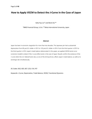
  • 6. Page 6 of 40 Figure 2.3 Demonstrates the relationship between trade balance of Japan and exchange rate of Japan. The trade balance of Japan declines after 2011. The foreign exchange reserves stays stagnant after 2012, so there should be no significant capital inflows to make the yen strong. Abe’s economic stimulus package hopes to stimulate the Japan's economy and improve its trade balance, which significantly depreciates the yen from 80 in 2012 to 120 in 2014. However, the trade balance declines, rather than increase, and the yen depreciate, Therefore, the J-curve phenomena occurs between 2012 Q3 and 2014Q3 (circle in Figure 2.3). From 2014 Q2 to 2015 Q4, Japan's trade balance and the yen depreciation improve from Abe’s economic stimulus package. Japanese firms conduct a strategic relocation of their production and a price-to-market (PTM) strategy so the export prices measured in contract (invoice) currency remain relatively stable since 2000, regardless of the exchange rate fluctuations. Therefore the export effects of the yen depreciation are mitigated. A weaker yen causes an increase in Japanese exports, but also induces imports of parts and components produced by Japanese overseas subsidiaries. Therefore, we could say that the depreciation of the yen would not make Japan's foreign exchange rate become an exogenous shock in the economy. Japan's foreign exchange rate is one of the endogenous variables for the trade balance model if there is no other significant driving force to make the foreign exchange rate become exogenous. After the Great East Japan Earthquake in March 2011, there was an increase in energy imports due to the shutdown of nuclear plant that causes a trade deficit for Japan. However, the oil price started to fall from the mid-2014 and the trade deficits improved. Abe’s economic stimulus package depreciates the
  • 7. Page 7 of 40 yen sharply from the end of 2012 and does not improve the trade balance in the first two years (2012 to 2014), but the trade balance truly improved from 2015 to 2016. Japanese firms conduct a relocation policy strategy to produce the low-end products overseas, and high-end products domestically. They conduct research and development (R&D) activities at the headquarters in Japan. Abe’s economic stimulus package would make Japanese firms become more inclined to accumulate as much earnings as possible from overseas assets as an income surplus, if the Japanese government implemented a tax exemption for foreign income. The Japanese economy should obtain more income effects for recovery from the income surplus. Figure 2.4 Demonstrates the relationship between trade balance of Japan and yearly growth of U.S GDP The significant growth of U.S GDP from 2012Q3 to 2014Q4 (circle in Figure 2.4) causes the strong expectation of an increase of the U.S. federal funds rate, which should be the exogenous shock to Japan's foreign exchange rate.
  • 8. Page 8 of 40 Figure 2.5 Demonstrates the economic interaction between foreign exchange rate of Japan and U.S Fed Funds rate. The United States is one of Japan's major trading partners, and the U.S. economy leads the Japanese economy. Interest rate is the instrument for the exchange rate. The U.S. federal funds rate is the real U.S. interest rate. The U.S. federal funds rate (interest rate) and Japan's foreign exchange rate are theoretically related by capital mobility. The U.S. federal funds rate leads the movement of Japan's foreign exchange rate. When the U.S federal funds rate increases, the yen depreciates. According to the Mundell-Fleming model, the increase of the U.S federal funds rate would attract more capital inflows to the United States from other countries including Japan. The impact of Japan's capital outflows would make the yen depreciate. Figure 2.5 demonstrates the yen depreciating to 120 per dollar when the U.S. federal funds rate reaches the peak at 5% from 2004 to 2008. When the U.S. federal funds rate stays low, from 2009 to 2012, the yen appreciates and hits a post war record high of 75.32 per dollar in October 2011. Abe’s economic stimulus package depreciates the yen sharply from the end of 2012, so the yen depreciated from 2012 to 2015 with low a U.S. federal funds rate. After 2015, the U.S. economy had a significant recovery and eliminated the risk of deflation, so the U.S. federal funds rate increases significantly. According to the base scenario of 2017 CCAR economic analysis, the U.S. federal funds rate will keep increasing from 2017 to 2019, which would cause the depreciation of the yen. Thus, the U.S. federal funds rate could be the major driving force that leads the trade balance of Japan.
  • 9. Page 9 of 40 Figure 2.6 demonstrates Japan's foreign exchange rate and a weighted average of the foreign exchange value of the U.S. dollar against the currencies of a broad group of major U.S. trading partners (US TRADEW) are co-integrated. TRADEW is a weighted average of the foreign exchange value of the U.S. dollar against the currencies of a broad group of major U.S. trading partners including Japan. The broad currency index includes the Euro Area, Canada, Japan, Mexico, China, United Kingdom, Taiwan, Korea, Singapore, Hong Kong, Malaysia, Brazil, Switzerland, Thailand, and the Philippines. Thus, TRADEW and Japan's foreign exchange rate are co-integrated and have the same movements. If the United States enhances business with its trading partners, Japan's economy should improve as well as other U.S. major trading partners. Figure 2.7 demonstrates the relationship between Japan's trade balance and the U.S. industrial production index (US IPI).
  • 10. Page 10 of 40 The U.S industrial Production index (U.S IPI) measures the real output produced by the manufacturing, mining, and electric and gas utilities industries in the United States, so the U.S IPI is considered to be the real production of the United States, which leads Japan's economy and the economy of other countries in the world. The U.S. IPI is sensitive to consumer demand and interest rates. Because the U.S. IPI is sensitive to demand, the U.S. domestic demand should increase along with the growth of the U.S IPI. The increase of U.S. domestic demand would enhance the trading between the United States and Japan. Thus, Japan's trade balance should improve. The U.S IPI starts to grow significantly since 2009. The growth of the U.S. IPI would lead the growth of the Japanese economy and enhanced the trade between U.S the United States and Japan. The U.S. IPI is the major driving force to lead the world economy. Japan's trade balance declined from 2012 to 2014 when the yen depreciates sharply due to Abe’s economic stimulus package. Figure 2.8 demonstrates the relationship between the U.S. IPI and the U.S. federal funds rate. The U.S. IPI is sensitive to the U.S. federal funds rate and has the same movements from 2003 and 2008. The U.S. federal funds rate is considered to be the United States' real interest rate. When the economy was overheated in 2006 and 2007, the U.S Federal Reserve’s bank had to increase the interest rate to avoid inflation. Because of the global financial crisis, the U.S. government tried to decrease the interest rate to stimulate the economy, which makes the U.S. federal funds rate close to zero from 2009 to 2015, with governmental intervention to stimulate U.S. IPI growth. The U.S. IPI did not grow, but declined with low interest rates, causing a risk of deflation in 2015. The U.S. Federal Reserve’s bank has to increase the interest rate to eliminate the risk of deflation in 2016. The base scenarios of the 2017 U.S Federal Reserve’s bank CCAR economic analysis demonstrates that the U.S Federal Reserve’s bank will continue
  • 11. Page 11 of 40 to increase the interest rate from 2017 Q1 to 2019 Q4, and the U.S. IPI should grow along with the rising interest rate. Figure 2.9 demonstrates the relationship between U.S IPI and U.S BBB Corporate risk spread U.S. credit spreads tend to widen during recession and to shrink during expansion. The credit spread is due to credit or default risk. The BBB rated bond is less during good economic times. The U.S. BBB corporate risk spread could be the measurement of industry risk. The higher the U.S. BBB corporate risk spread is, the lower U.S. industry production is supposed to be. The U.S. BBB corporate risk spread reached its peak in the global financial crisis period, so U.S. industry productions touch the trough during that period. The economic analysis of 2017 CCAR indicates that U.S. industrial production would grow significantly with the low risk index of the U.S. BBB corporate risk spread.
  • 12. Page 12 of 40 Figure 2.10 demonstrates the CCAR economic scenarios of GDP of Japan. Japan has been in a recession for more than twenty years. The scenarios of the 2017 CCAR economic analysis indicates that Japan's GDP would grow strongly. There are a few reasons to that would make Japan's GDP obtain significant growth after the end of 2016. For example, the recovery of the U.S. economy could cause the growth of the Japanese economy, so Japan's GDP would grow. Abe’s economic stimulus package enhances the trading with the Japan's trading partners after 2015. This stimulus makes Japanese firms become more inclined to accumulate as much earnings of overseas assets as possible as income surplus if the Japanese government implemented a tax exemption for foreign income. Japan's economy would obtain more capital for growth and then obtain significant growth of the GDP. Different from the stagnant GDP before 2014, the growing GDP of Japan would become the driving force of the trade balance model. III Data and Methodology Quarterly data from Japan’s trade balance, the U.S industrial production index and Japan’s foreign exchange rate were collected from various sources. The quarterly data from Japan's trade balance came from the Bank of Japan. The U.S. industrial production index and Japan's foreign exchange rate came from U.S Federal Reserve's Bank. The data for model specification spans from 2003Q1 to 2016Q3, which includes the period of the Global Financial Crisis (2008Q3-2010Q4) as well as the period of the recovery (2011Q4-present). This paper includes the stress testing of Japan's trade balance, where the driving forces of the Vector Error Correction Model (VECM) came from the U.S. Federal Reserve Bank’s 2017
  • 13. Page 13 of 40 CCAR. The driving forces are exogenous and the major driving forces for Japan's trade balance are the U.S federal funds rate, the U.S. BBB corporate risk spread, Japan's GDP and TRADEW (a weighted average of the foreign exchange value of the U.S. dollar against the currencies of a broad group of major U.S. trading partners. The data for the economic analysis covers the periods of the Japanese recession in the 1990s, the Global Financial Crisis and recovery of the economy. Japan is one of the most developed countries in the world and relies on imports from other developed countries. Japanese firms implement a strategic relocation of their production and price-to-market (PTM) strategy to resolve the fluctuation of exchange rate for more than 10 years. Although Abe’s economic stimulus package depreciates the yen sharply, from 80 in 2012, to 120 in 2014, the depreciation of the yen might not improve the trade balance significantly in the short run. Japan's trade balance decreased rather than increased from 2012 to 2014. However, Japan’s trade balance improved after 2015. As one of Japan's major trading partners, the U.S economy leads Japanese economy. Japan's economy improved when U.S economy turns better. This paper demonstrates the trade balance model between the United States and Japan. The J-Curve phenomena cause currency depreciation, improve the trade balance in the long run, but worsen the trade balance in the short run. The trade balance model from Rose and Yellen (1989) indicates that the trade balance is the function of exchange rates and incomes of trade partners. The trade balance models would be demonstrated as follows: TB = X·Px - M·Pm = TB (q, Yx, Ym) Equation (3.1) Where TB: trade balance of Japan X: export demand of Japan Px: price of export Pm: price of import M: import demand of Japan Yx: real income of export country Ym: real income of import country q: exchange rate
  • 14. Page 14 of 40 Equation 3.1 demonstrates the outline of the trade balance model. If we focus on the trade balance model between the United States and Japan, it would become the function of the exchange rate (yen/dollar), Japan's industrial production index (JapanIPI), and the U.S. industrial production index (USIPI). This paper employs the industrial production index to be the real GDP. Since the United States is one of the major trading partners of Japan, the trade balance between Japan and the United States should be significantly co-integrated with Japan's total trade balance. Thus, this paper uses Japan's aggregate trade balance in the trade balance model between Japan and the United States. Because Japan has been in a recession for more than twenty years, Japan's industrial production index did not obtain significant growth and remained stagnant during the recession period. Japan's stagnant industrial production index would cause a collinear problem in the trade balance model, so we have to exclude it.. The revised trade balance model between the United States and Japan should look like Equation (3.2): JAPANTB = TB (EXJAPAN, USIPI) Equation (3.2) Equation 3.2 demonstrates the long-run economic interactions of endogenous variables, which includes the Japan's foreign exchange rate (yen/dollar), and the U.S industrial production index as endogenous variables. Japan's government is the central planer who tries to maximize the utility of the trade balance to reach the Pareto optimality condition of the economy. According to the second welfare theorem, the Pareto optimality of the economy would lead to a competitive equilibrium. Thus, agents would maximize their utilities; firms would maximize their profits and the market would clear. The Pareto optimality could be demonstrated in the following mathematic optimization form: Mathematic optimizations: MAX {U (USIPI, EXJAPAN)} s.t. β0 + β1·USIPI + β2·EXJAPAN < = C £ = U + λ· (C- (β0 + β1·USIPI+ β2·EXJAPAN)) F.O.C: ∇USIPI, EXJAPAN, λ £ (USIPI, EXJAPAN, λ) = 0 Note that ∇ λ £ (USIPI, EXJAPAN, λ) = 0 means β0 + β1·USIPI + β2·EXJAPAN = C Where
  • 15. Page 15 of 40 U (JAPANTB): utility of central planner for trade balance U (JAPANTB) =U (EXJAPAN, USIPI) JAPANTB: the trade balance of Japan USIPI: US industrial production index EXJAPAN: exchange rate of Japan (yen/dollar) C: constant level of trade balance; C > 0 Milton Friedman said that the best model should be the model that provides the best forecasts. This should hold when the model achieves the Pareto Optimality. Both the multivariate time-series model (VECM) and mathematic optimization demonstrates the framework of Pareto Optimality. Specifically, the multivariate time-series model accommodates the impacts of exogenous shocks and uses the resources to maximize the utility of the central planner so that the Pareto Optimality is achieved. For the trade balance model, the central planner is maximizing utility of the central planner subject to the trade balance constraint of endogenous variables. However, the driving forces (exogenous shocks or predetermined variables) would lead the model to obtain the best forecasts. Budget constraint ensures economic interactions of endogenous variables in the steady state (long-run equilibrium). The first order conditions of the above optimization demonstrate that there is no weakly exogenous or exogenous condition of endogenous variables in the transitional dynamics (short-run equilibrium). The exogenous variables are the driving forces, which are the shocks of the model. The shocks would cause the model to deviate from a steady state. A variable cannot be endogenous and exogenous variable at the same time. Based on the concept of the mathematic optimization, we specify the trade balance model in the following steps: Step 1: We construct an ordinary least square model (OLS) as the baseline model to identify the co- integration relationship (steady state or long-run equilibrium) of the endogenous variables and specify the impulse indicators to capture the hit-and-run impacts of the exogenous shocks. JAPANTB = β0 + β1·EXJAPAN + β2·USIPI + β3·IDUM1 + β4·IDUM2 + β5·IDUM3 + u Equation (3.3) Where
  • 16. Page 16 of 40 IDUM1: the impulse indicator captures the uptrend impacts of exogenous shocks IDUM2: the impulse indicator captures the downtrend impacts of exogenous shocks IDUM3: the impulse indicator captures the specific outlier impacts of exogenous variables u: the error terms; the error terms need to be white noise that indicates zero mean, normally distributed and, no serial correlation of the error term Equation 3.3 indicates the model is deviating from the steady state when impulse indicators are significant. The impulse indicators are a type of additive dummies that take a value of “0” or “1.” They are called “on” or “off” variables, where “1” corresponds to “on”. The impulse indicators capture the impacts of the exogenous shocks, which ensure the stabilities of parameters and white noise error terms when the model is deviating from the steady state. The impacts of the exogenous shocks come from the effects of policy changes, company mergers, regulation changes, and financial crises, etc. The impulse indicators exclude the non-linear issues from the exogenous shocks. Ignoring the impulse indicators, the information set would be asymmetric and the model would be incorrectly specified. JAPANTB = β0 + β1·EXJAPAN + β2·USIPI + є Equation (3.4) Where refers the error term of the co-integration equation. Equation 3.4 demonstrates the co-integration relationship (steady state or long-run equilibrium) of endogenous variables in the trade balance model, which includes Japan's trade balance, foreign exchange rate and the U.S industrial production index. The definition of co-integration indicates that all endogenous variables do not have to be stationary, but the first difference of the endogenous variables, and the linear combination of the endogenous variables (error terms) must be stationary. The OLS methodology identifies the steady state the model is approaching, and specifies the impulse indicators needed to capture the hit-and-run impacts of shocks. However, OLS is not able to demonstrate the economic interactions in the transitional dynamics and judge the driving forces to restore (or deviate) the model back to the steady state. This paper is investigating the trade balance model between Japan and the United States. The U.S. economy leads Japan's economy so the U.S. economic indices should be the driving forces to lead the trade balance model back to a steady state. It is important to know under what conditions a real depreciation of the yen improves Japan's trade balance of Japan in the long run, but worsens it in the
  • 17. Page 17 of 40 short run. Abe’s economic stimulus package depreciates the yen sharply when the Japan's economy is in a recession. This paper determines if the impacts of the yen depreciation are significant enough to make Japan's foreign exchange rate cause exogenous shocks in the model, which are the J-curve phenomena. In order to demonstrate the above economic activities, we apply the multivariate time series model (VECM) in the step 2. Step 2: We run the VECM to demonstrate the economic activities in the steady state, and also in the transitional dynamics. Equation 3.5 demonstrates the VECM. ΔZ𝑡+1 = C + Σ Гi ΔZ𝑡−𝑖 +αβ’ Z𝑡 + ΦD𝑡 + δΔHt+1 + ε𝑡; i= 1, 2 …...... Equation (3.5) In the trade balance model of Japan, the lag of VAR is one. Thus, i=1 Zt: the vector of endogenous variables that are JAPANTB (trade balance of Japan), EXJAPAN (foreign exchange rate of Japan, and USIPI (U.S industrial production index) β: long run parameter Beta estimates (co-integrating vector) α: adjustment coefficient Alpha estimation (error correction vector) β'Zt-1: the vector of co-integrating vector αβ'Zt-1: the lagged error correction term in VECM ΔZt: the vector of the first difference of endogenous variables ΔHt+1: the first difference of risk factors (or predetermined variables); the significant change of risk factors are exogenous shocks (DJGDP, DTRADEW, DUSBBBCORPRISKSPREAD, and DUSFEDFUNDSRATE) Dt: Dt includes the impulse indicators (IDUM1 IDUM2 and IDUM3) and driving forces (DJGDP, DTRADEW, DUSBBBCORPRISKSPREA, and DUSFEDFUNDSRATE) Єt: the error terms of transitional dynamics of VEC, which need to be white noise DJGDP: the first difference of GDP of Japan DTRADEW: the first difference of a weighted average of the foreign exchange value of the U.S. dollar against the currencies of a broad group of major U.S. trading partners
  • 18. Page 18 of 40 DUSBBBCORPRISKSPREA: the first difference of U.S corporate risk spread DUSFEDFUNDSRATE: the first difference of U.S federal funds rate The Dt of the VECM includes all exogenous factors that are dummy variables (or impulse indicators) and driving forces (predetermined variables). The exogenous driving forces (shocks) could provide the impacts to efficiently restore the model back to the steady state when the economy condition is turning better. The results of Granger causality could provide the candidates of driving forces. It is very important to identify the economic condition and select the correct driving forces for the VECM. All of the endogenous variables move simultaneously in the VECM. When we select driving forces, we have to consider the driving forces for all endogenous variables, not only those for the objective (normalized) variable in the VECM. All transitional dynamics of endogenous variables of the VECM should exclude the weakly exogenous. The growth of the U.S economy picks up in 2012Q3 and advances above the 4% annualized rate for several quarters. The strong recovery of the U.S .economy would cause the strong expectation of a rise in the U.S federal funds rate. During the recession period, U.S. and Japanese interest rates are very low and even low enough to cause the risk of deflation. Interest rates are the instrument for the exchange rate because interest rates and exchange rates are related for capital mobility. The strong expectation of the increase of the U.S. federal funds rate would affect Japan's foreign exchange rate as well as its trade balance. Interest rates could affect the trade balance if international substitution influences consumption and imports. The U.S. federal funds rate is considered as the real interest rate of the U.S. economy. The efficient recovery of the U.S. economy would push the rise of the U.S. federal funds rate, which would cause more capital inflow to the United States from Japan and other countries in the world. The significant capital inflow would make the U.S. dollar stronger and make the yen weaker. Thus, the U.S. federal funds rate should be one of the major driving forces of trade balance model between Japan and the United States. The base scenario of 2017 CCAR economic analysis demonstrates that Japan's GDP will be no longer stagnant, and grow significantly after 2016 Q3 to 2019Q4. Thus, Japan's GDP should be the driving force of the trade balance model to mutually improve U.S. and Japanese industrial production. TRADEW is a weighted average of the foreign exchange value of the U.S. Dollar against the currencies of a broad group of major U.S. trading partners, including Japan. When the Dollar becomes strong, TRADEW would become depreciated and enhance the worldwide trading business. Therefore TRADEW is selected to be one of the driving forces. The U.S. BBB corporate risk spread would affect the
  • 19. Page 19 of 40 U.S. industrial production index; therefore this is also selected as one of the driving forces for the trade balance model. Most of the previous studies used log-level data. However, in order to keep the nature of data, the baseline OLS model regression is run with data in level without any data transformation. In order to satisfy the definition of the co-integration, the first difference of endogenous variables and the error term of co-integration equation have to be stationary. A constant is estimated in OLS and the VECM models because Japan's trade balance data shows a deterministic drift. Japan's trade balance data demonstrates certain specific patterns, but not significant enough to be called seasonal patterns. We incorporate these patterns in the impulse indicators both in-sample and out-of-sample. The forecasts are based on the historical information set. If the historical information set demonstrates the specific patterns of data nature, the similar patterns would show up in the future economic activities (forecasts). Therefore, we have to understand the data nature carefully to specify the impulse indicators both in- sample and out-of-sample. Under such conditions, we will avoid using too many dummy variables that would cause the collinear problems. The VECM trade balance model only has one lag. The number of lags should be less than four (there are four quarters in a year) for a well-specified model if the data of all endogenous variables are independent and identically distributed random variables. Most previous papers specify the trade balance model as the following two equations: The first equation of the model demonstrates the baseline OLS model regression. However, without imposing any impulse indicators to capture the impacts of exogenous shocks, the model should be miss- specified and provide the spurious results to demonstrate economic interactions of endogenous variables. The second equation demonstrates the transitional dynamics by using ARDL (auto-regression distribution lag) model. However, the second equation makes endogenous variables, except TB, be exogenous shocks as well. There is no impulse indicator to capture the impacts of exogenous shocks. No variable can be endogenous and exogenous at the same time in the transitional dynamics. This paper revises the model and presents better economic intuitions.
  • 20. Page 20 of 40 IV. Empirical Results The J-curve phenomena indicate that currency depreciation improves the trade balance in the long-run, but worsens it in the short run. However, the existence of the J-curve phenomena is in debate. Rose and Yellen (1989) state no statistically reliable evidence of a stable J-curve is detected when they did research on the U.S. trade balance model. Rose and Yellen (1989) emphasize that if ordinary least square (OLS) is used, weak evidence of a J-curve is detected. They also question under what circumstances a real depreciation improves the real trade balance in the long run and worsen it in the short run. The J-curve phenomena might occur when there is a certain factor or issue to cause the exchange rate of trade balance model from endogenous to exogenous, which makes the exchange rate a significant shock to the trade balance. The most previous studies applied both the OLS and auto- regressive distribution lag (ARDL) models to demonstrate that the economic activities of the trade balance model in the long run equilibrium and in the short run dynamics. However, this methodology is not able to demonstrate the economic activities in transitional dynamics precisely. This paper applied both the OLS model and the VECM. The OLS model is the baseline model to specify the co-integration equation and demonstrate the economic activities of endogenous variables in the long run. The VECM demonstrates that the economic activities in the steady state and in the transitional dynamics. The results are shown in the followings: Table 4.1 demonstrates the results of OLS model
  • 21. Page 21 of 40 Table 4.1 demonstrates high R-square value (0.9517) of the OLS model, which presents the Goodness-of Fit for the model. The values of VIF (variance inflation) for all variables are less than 3 and the co- linearity diagnostic index are less than 100, so there are no multi-collinearity and collinear problems in the model. The multi-collinearity and collinear problems occur because endogenous variables obtain a certain degree of identical information between each other, which would cause the singular problem of the model and even make the model break down. All independent variables are significant. The results of OLS model indicate Japan's trade balance moves positively when the U.S. industrial production index (USIPI) grows significantly; Japan's trade balance moves gradually when its foreign exchange rate depreciates significantly. USIPI and EXJAPAN are endogenous in the model. The depreciation from Abe’s economic stimulus package would not be strong enough to cause Japan's foreign exchange rate (EXJAPAN) to be exogenous. The impulse indicators (IDUM1, IDUM2 and IDUM3) are exogenous to capture the impacts of exogenous shocks, which indicate the model is deviating from the steady state. The function of an impulse indicator is to stabilize the parameters and capture the hit-and-run impacts in the face of exogenous shocks. The OLS model helps to define the steady state of trade balance model and to specify the impulse indicators when the model is deviating from the steady state. The results of applying the OLS model demonstrates that Japan’s trade balance would move positively and its foreign exchange rate would depreciate in the long run. Rose and Yellen (1989) indicate “a J-curve is defined as the combination of a negative short-run derivative with a positive long-run derivation. The question posed-under what circumstances a real depreciation improves the real trade balance in the long run but worsen it in the short run --- is distinctly partial equilibrium in nature”. We apply the VECM to discuss the J-curve in detail after we specify the baseline OLS models. The results of the VECM are as follows:
  • 22. Page 22 of 40 Table 4.8 demonstrates the steady state (co-integration equation or the long-run equilibrium) of VECM We identify the steady state of the trade balance model and test the co-integration (Appendix 1). The long run equilibrium (co-integration or steady state) of the VECM demonstrates JAPANTB - 65.43019·USIPI – 74.0087·EXJAPAN=0. Because the application of the impulse indicators in the VECM provide a complete information set, the sign of parameters of independent variables are correct. The steady state indicates that Japan’s trade balance would increase gradually and its foreign exchange rate would depreciate while the U.S industrial production index would expand in the long run. The steady state provides the reliable and stable economic interactions of endogenous variables. Table 4.9 demonstrates the transitional dynamics of the objective function JAPANTB in the VECM The objective variable of the trade balance model is JAPANTB, so we normalize JAPANTB in the VECM. The VECM makes all endogenous variables move simultaneously in response to the exogenous shocks in the transitional dynamics. We should select the driving forces for all endogenous variables. Driving forces (predetermined variables) are the exogenous shocks. According to the efficient recovery of U.S
  • 23. Page 23 of 40 economy, the United States would increase the federal funds rate. However, it is important to determine if the Federal Reserve’s Bank increases the U.S federal funds rate too much and too fast to make Japan’s foreign exchange rate become exogenous shock in the trade balance model. The U.S. federal funds rate and U.S. BBB corporate spread risk are the major driving forces of JAPANTB. The transitional dynamics of JAPANTB show the shock impacts of the U.S. federal funds rate and U.S. BBB Corporate risk spread would cause the decline of JAPANTB significantly. JAPANTB is the objective variable in the trade balance model. We observe that the JAPANTB sustains the impacts of exogenous shocks in transitional dynamics and that there is no issue with having weakly exogenous for endogenous variables (USIPI and EXJAPAN) because there is no significant shock impact of USIPI and EXJAPAN on JAPANTB in the previous period (t-1). The VECM provides the information to detect when other endogenous variables (EXJAPAN and USIPI) will become exogenous under certain conditions. When the objective variable (JAPANTB) and other endogenous variables (EXJAPAN and USIPI) are affected by the same driving force in the VECM simultaneously, the impacts of a driving force would make that endogenous variable turn exogenous to affect JAPANTB implicitly. This demonstrates the existence of a J-curve in the trade balance model. This paper will discuss this issue in the following transitional dynamics. Table 4.10 demonstrates the transitional dynamics of EXJAPAN in the VECM The transitional dynamics of EXJAPAN provides the forecast of EXJAPAN and also demonstrates when EXJAPAN would become exogenous to JAPANTB under certain condition. TRADEW and the U.S. BBB corporate risk spread are major driving forces for EXJAPAN in the transitional dynamics. The shock
  • 24. Page 24 of 40 impacts of the U.S. federal funds rate on EXJAPAN are almost significant. There is no weakly exogenous issue of endogenous variables (JAPANTB and USIPI) on EXJAPAN. The shock impacts of depreciated TRADEW would cause the depreciation of the yen to compete with Japan’s trade partners. The shock impact of a rising U.S. BBB corporate risk spread indicates more risk in the U.S. economy would cause more capital outflows from the United States to Japan and push the yen appreciated. The shock impacts of a rising U.S .federal funds rate would cause more capital inflows to the United States from Japan and make the yen depreciated. However, the U.S. federal funds rate is the driving force that affects JAPANTB and EXJAPAN simultaneously in the transitional dynamics. EXJAPAN would become exogenous to the trade balance model when the shock impacts of U.S. federal funds rate affects EXJAPAN significantly, and make EXJAPAN exogenous in the transitional dynamics. Interest rates are the instrumental variable for the exchange rate. As long as the shock impacts of the U.S. federal funds rate affect EXJAPAN significantly, EXJAPAN would change from endogenous to exogenous in the trade balance model implicitly. The following equations demonstrate how the U.S. federal funds rate would become the driving force to make EXJAPAN become exogenous in the trade balance model. Equation 4.1 demonstrates Japan’s trade balance (JAPANTB) as the function of Japan’s foreign exchange rate (EXJAPAN) and the U.S. industrial production index (USIPI). Equation 4.2 indicates EXJAPAN is the function of U.S federal funds rate if we specify EXJAPAN individually. The shock impacts of the U.S federal funds rate would affect JAPANTB and EXJAPAN. However, when the shock impacts of the U.S federal funds rate affect EXJAPAN significantly, EXJAPAN would turn from endogenous to exogenous and affect JAPANTB implicitly. Equation 4.3 demonstrates the relationships between JAPANTB, the U.S. federal funds rate and EXJAPAN. The shock impact of the U.S. federal funds rate on JAPANTB is negative (Table 4.9) and the shock impact of the U.S. federal funds rate on EXJAPAN is positive (Table 4.10). Thus, the shock impact of EXJAPAN on JAPANTB should be negative in the transitional dynamics, which is the J-curve phenomenon in the trade balance model. Because the U.S. Federal Reserve’s Bank will not
  • 25. Page 25 of 40 increase the interest rate dramatically, we believe the impacts of the U.S. federal funds rate on EXJAPAN will be mitigated and become insignificant. Thus, EXJAPAN is still an endogenous variable in the model. From the above, we could say the J-curve phenomenon occurs when the shock impacts of the U.S. federal funds rate affect JAPANTB and EXJAPAN in the transitional dynamics simultaneously. Under such conditions, EXJAPAN would turn from endogenous to exogenous in the trade balance model. Rose and Yellen (1989) states “The question posed-under what circumstances a real depreciation improves the real trade balance in the long run but worsen it in the short run --- is distinctly partial equilibrium in nature”. The transitional dynamics of all endogenous variables in the VECM demonstrates the question of "partial equilibrium in nature" of Rose and Yellen (1989). Table 4.11 demonstrates the transitional dynamics of USIPI The transitional dynamics of USIPI provides the forecast of USIPI and also demonstrates when USIPI would become exogenous in the trade balance model. Japan’s GDP (JGDP) and the U.S. BBB corporate risk spread are major driving forces for USIPI in the transitional dynamics. The shock impacts of the U.S. BBB corporate risk spread on USIPI are significant. There is no weak exogenous issue of endogenous variables (JAPANTB and EXJAPAN) on USIPI asymptotically. The shock impacts of a rising U.S. BBB corporate risk spread indicates more risk in the U.S. economy, which would lower the U.S. industrial production index (USIPI). The shock impacts of an improved Japanese GDP and would enhance the U.S .industrial production index (USIPI). However, the U.S. BBB corporate risk spread is the driving force for JAPANTB and USIPI in the transitional dynamics. USIPI
  • 26. Page 26 of 40 would become an exogenous variable in the trade balance model when the shock impacts of the U.S. BBB corporate risk spread affect USIPI significantly. If we specify the USIPI model individually, USIPI should be the function of the U.S. BBB corporate risk spread (Equation 4.4). As long as the shock impacts of the U.S. BBB corporate risk spread affect USIPI significantly, USIPI would change from endogenous to exogenous in the trade balance model to affect JAPANTB implicitly. The following equations demonstrate how the U.S. BBB corporate risk spread would become the driving force to make USIPI become exogenous in the trade balance model. Equation 4.1 demonstrates Japan’s trade balance (JAPANTB) is the function of the U.S. industrial production index (USIPI). Equation 4.4 indicates USIPI is the function of the U.S. BBB corporate risk spread if we specify USIPI individually. Equation 4.5 shows how the shock impacts of USIPI would affect JAPANTB when the shock impacts of the U.S. BBB corporate risk spread affect USIPI and turn USIPI to exogenous shock in the trade balance model. Equation 4.5 demonstrates the implicit relationships between JAPANTB, the U.S. BBB corporate risk spread and USIPI. The shock impact of the U.S. BBB corporate risk spread rate on JAPANTB is negative (Table 4.9) and the shock impact of the U.S. BBB corporate risk spread on USIPI is negative (Table 4.11). Thus, the shock impact of USIPI on JAPANTB should be positive in the transitional dynamics, which is the implicit impact of the U.S. BBB corporate risk spread on the trade balance model. We believe the U.S. economy will continue to improve, so the impacts of the U.S. BBB corporate risk spread on endogenous variables will be mitigated. Thus, we keep USIPI in the model. V. Conclusion Japan has been in a recession for more than twenty years. In order to get out of the recession, the government of Japan tried to lower interest rate and implement monetary expansion. Many economists wondered whether the accommodative policy would induce exchange rate depreciation, which might shift the aggregate demand through improvement of net exports. Abe’s economic stimulus package planned to stimulate Japan’s economy and improve the its trade balance, which makes the yen
  • 27. Page 27 of 40 significantly depreciated from 80 in 2012 to 120 in 2014. However, the trade balance did not improve, it declined, with the depreciation of the yen between 2012 Q3 and 2014Q3. Therefore the J-curve phenomena occurred, which indicates that currency depreciation improves the trade balance in the long-run, but worsens it in the short run. However, the existence of J-curve phenomena is in debate. Most previous studies applied both the OLS and ARDL (auto-regressive distribution lag) models to demonstrate the economic activities of trade balance model in the long run equilibrium and in the transitional dynamics, which emphasize the J-curve in the sample size period. We are not able to judge the impacts of exogenous shocks (driving forces) in the previous studies. However, this methodology is not good enough to demonstrate the economic interactions between endogenous variables and exogenous shocks in the transitional dynamics. The ARDL model they applied is not able to provide forecasts of endogenous variables nor could it detect the J-curve under certain conditions in the transitional dynamics. This paper applied OLS model as the baseline model to specify the steady state and impulse indicators. Different from the previous studies, we applied the VECM (Johansen 1995) not the ARDL model to detect a J-curve. The results of the VECM model demonstrate the economic interactions between endogenous variables and exogenous shocks in the transitional dynamics. We found that the J-curve phenomena occurs when one driving force (the U.S. federal funds rate) affects more than one endogenous variable (Japan’s trade balance (JAPANTB) and Japan’s foreign exchange rate (EXJAPAN)) simultaneously in the transitional dynamics, the shock impacts of the U.S. federal funds rate would affect the Japan’s foreign exchange rate (EXJAPAN) and turn it to an exogenous shock on Japan’s trade balance (JAPANTB) implicitly. The J-curve phenomena occur under such conditions. The stress test results of driving forces provide the forecasts to lead the expectation of economic activities. The concept of new classical economics indicates the rational expectation leads to economic activities. The rational forecasts of the U.S. federal funds rate would lead the economic interactions of trade balance model in the transitional dynamics. If the U.S. Federal Reserve’s Bank raises the U.S. federal funds rate gradually but not dramatically, the U.S. federal funds rate would not make Japan’s foreign exchange rate be an exogenous shock to affect Japan’s trade balance in the near future (2017 to 2019). The same situation occurs when the same driving force affects the objective variable and other endogenous variables simultaneously in the transitional dynamics. The specific driving force would turn that endogenous variable to an exogenous variable to affect the objective variable. However, these impacts could be mitigated with the appropriate policies or actions on the driving forces.
  • 28. Page 28 of 40 Although Japanese firms implemented a strategic relocation of their production and price-to-market (PTM) strategy to overcome the foreign exchange rate fluctuation, the significant depreciation of the yen would cause the endogenous and even exogenous impacts on the Japan’s trade balance. Interest rates are the instrument for the exchange rate because interest rates and exchange rates are related to capital mobility. The significant growth of the U.S. GDP from 2012Q3 to 2014Q4 leads the strong expectation of an increase of the U.S federal funds rate. Even the U.S. federal funds rate did not rise too much from 2012 to 2014. However, the expectation of the increase of the U.S. federal funds rate was very strong at that time. The longer the interest rate stays close to zero, the more sensitive the interest rate would rise (Appendix Figure A3.1). The expectation of interest rate-led economic activities at that period and the shock impacts of the U.S. federal funds rate on the foreign exchange rate make the J- curve phenomena occur from 2012 to 2014. The shock impacts of the U.S. federal funds rate would be mitigated and not significantly affect the foreign exchange rate, so the J-curve phenomena was mitigated. Rose and Yellen (1989) state no statistically reliable evidence of a stable J-curve is detected when they did research on the U.S. trade balance model. They also question whether the OLS model is good enough to detect the J-curve. The J-curve might occur under certain circumstances in the short run. The question posed-under what circumstances a real depreciation improves the real trade balance in the long run but worsen it in the short run --- is distinctly partial equilibrium in nature. The OLS model is a static model to present the steady state in the long run. However, the J-curve phenomena occurs in the transitional dynamics (in the short run), which should be detected by using the VECM (Johansen 1995). Thus, the OLS model is not able to detect the J-curve. Rose and Yellen (1989) did research on trade balance model before the VECM (1995) was well developed, so they were not able to detect a J-curve. However, the questions they pointed out lead us to accomplish our work in this paper.
  • 29. Page 29 of 40 Compliance with Ethical Standards: Conflict of Interest: I _____KELLY YIYU LIN_______________- as corresponding author, certify that all authors contributed significantly to the manuscript and no other authors were involved and were not part of the team that created this manuscript. All used data are correct and results are based on authors’ calculations. Author(s) is/are solely responsible for the entire content and results of the paper published in the journal. I certify that no part of this manuscript has been published before or is not under consideration for publication elsewhere. I certified that this manuscript was used as working paper only. Title of the manuscript Does the J-Curve Exist? An Investigation in the Case of Japan Authors’ name / affiliation / official email address Percentage of contribution 1. KELLY YIYU LIN 70% 2.WENTI DU 30% Ethical Approval: This article does not contain any study
  • 30. Page 30 of 40 References: Akram, T. (2016). Japan's Liquidity Trap. Levy Economics Institute of Bard College Working Paper No. 862. Anderson, D., Botman, D., & Hunt, B. (2014). Is Japan’s Population Aging Deflationary? IMF Working Paper WP/14/139. Bernanke, B. S. (2000). Japanese monetary policy: a case of self-induced paralysis? Japan’s financial crisis and its parallels to US experience, 149-166. Bahmani-Oskooee, M. Mohsen and Gour G. Goswami (2003) "A Disaggregated Approach to Test the J-Curve Phenomenon: Japan versus Her Major Trading Partners," Journal of Economics and Finance, 27(1), pp.102-113. Bahmani-Oskooee, M. Mohsen and Artatrana Ratha (2004) “The J-curve: A Literature Review,” Applied Economics, 36, pp.1377-1398. Doi, T., Hoshi, T., & Okimoto, T. (2011). Japanese Government Debt and Sustainability of Fiscal Policy. Journal of the Japanese and International Economies, 25, 414-433. Eggertsson, G. B., & Krugman, P. (2012). Debt, Deleveraging, and the Liquidity Trap: A Fisher-Minsky-Koo Approach. The Quarterly Journal of Economics, 127(3), 1469-1513. Engle, R. F. (1982). Autoregressive Conditional Heteroscedasticity with Estimates of the Variance of United Kingdom Inflation. Econometrica, 50(4), 987. Engle, R. F. & Granger, C. W. J. (1987). Co-integration and error correction: Representation, estimation and testing. Econometrica, 55(2), 251–276. Granger, C. (1981). Some properties of time series data and their use in econometric model specification. Journal of Econometrics, 16(1), 121-130. Hendry, David.F & Santos, Carlos (2005), Regression Models with Data-Based Indicators Variables. Oxford Bulletin of Economics and Statistics, Volume 67, Issue 5, 571-595. Hoshi, T., & Ito, T. (2014). Defying gravity: can Japanese sovereign debt continue to increase without a crisis? Economic Policy, 29 (77), 5-44. Ihori, T., Kato, R. R., Kawade, M., & Bessho, S. (2006). Public Debt and Economic Growth in an Aging Japan. Tackling Japans Fiscal Challenges, 30-68. Johansen, S. (1992). Cointegration in partial systems and the efficiency of single-equation analysis. Journal of Econometrics, 52(3), 389-402. Johansen Søren.(1995) Likelihood-Based Inference in co-integrated vector auto-regressive models, Oxford University Press
  • 31. Page 31 of 40 Keynes, J.M. (2007). General Theory of Employment, Interest, and Money. New York, NY: Macmillan. Krugman, P. (1998). Japan’s Trap. Retrieved July 27, 2017, from http://web.mit.edu/krugman/www/japtrap.html Rose, A.( 1990) Exchange rates and the trade balance: Some evidence from developing countries, Economics Letters, 34, no. 3, 271-275. Rose, A.( 1991) The role of exchange rates in a popular model of international trade: Does the ' Marshall-Lerner' condition hold?, Journal of International Economics. 30, nos. 3-4, 301-315. Rose, A. and J. Yellen (1989) Is there a J-curve?, Journal of Monetary Economics 24, no. 1 , 53-68. Shimizu Junko and Sato Kiyotaka , Abenomics, Yen Depreciation, Trade Deficit, and Export Competitiveness, The Research Institute of Economy, Trade and Industry (http://www.rieti.go.jp/en/)
  • 32. Page 32 of 40 Appendix: Appendix 1: The Results of OLS Model and Co-integration Test The Results of OLS Model: Table A1.1 demonstrates the statistics of Durbin-Watson and autocorrelation check for white noise.
  • 33. Page 33 of 40 TableA1.1 demonstrates the statistics of Durbin-Watson is 2.052 (greater than 1.8 but less than 2.2) and the P-value of autocorrelation check for white noise is greater than 5% so there is no serial correlation between the residuals of the model. Table A1.2 demonstrates the error terms of the model are normally distributed Table A1.2 shows the error terms have zero mean and the p-value of Anderson-Darling of normality test is greater than 5%, so the error terms of the model are normally distributed. The normally distributed error terms indicate the stability of parameters of the model, which ensures there is no nonlinear issue of the model in the face of exogenous shocks. In the face of exogenous shocks, the error terms could be serial correlated and non-normally distributed. The serial correlation of the error terms would cause the biased in-sample economic analysis and out-of- sample forecasts. The non-normally distributed error terms would cause the instabilities of parameters, which would generate either under-forecast or over-forecast results. From the above statement, the error terms are normally distributed with zero mean and there is no serial correlation of the error terms so the error terms are white noise and the model is well-specified.
  • 34. Page 34 of 40 Table A1.3 demonstrates the error terms are not correlated with any independent variables. The independent variables are not correlated with the error terms, so Japan’s trade balance is fully explained by the independent variables. Co-integration Test of the endogenous variables: The definition of co-integration indicates that the endogenous variables do not need to be stationary, but the first differences of endogenous variables must be stationary and the residuals of co-integration equation must be stationary.
  • 35. Page 35 of 40 Table A1.4 demonstrates the economic interactions of co-integration equation The co-integration equation does not incorporate the impulse indicators, so the information set of co- integration equation is incomplete (asymmetric), which does not include the hit-and-run impacts of the exogenous shocks. Because of the incomplete information set of co-integration equation, the results show incorrect sign of the estimate of USIPI, which is spurious and different from the results of the previous well-specified OLS model. The OLS model was therefore applied to specify the steady state (Long-run equilibrium). Table A1.5 demonstrates the level data of endogenous variables are not stationary
  • 36. Page 36 of 40 Table A1.6 demonstrates the first differences of endogenous variables are stationary and the residuals of co-integration equation (RES) is stationary Although the result of first lag of residuals of co-integration equation is semi-stationary, in the long run, the residuals would be stationary. Figure A1.7 demonstrates the actual and prediction values of trade balance of Japan Without any collinear or multicollinearity problems of the model, the model is well-specified and satisfied Goodness-of-fit. The regression results are highly co-integrated with the actual value of Japan’s trade balance.
  • 37. Page 37 of 40 Appendix 2: Results of the VECM Table A2.1 demonstrates the error terms of transitional dynamic equations of the VECM are normally distributed with zero mean Table A2.1 demonstrates the error terms of transitional dynamic equations of the VECM are normally distributed. Thus, the parameters of transitional dynamic equations are stable, and there is no nonlinear issue in the transitional dynamic equations. Table A2.2 demonstrates the error terms of transitional dynamic equations of the VECM are not serial correlated (P-value >5%) The above results demonstrate the error terms of transitional dynamics of the VECM are white noise. Figure A2.1 demonstrates The Error Correction Vector (α)
  • 38. Page 38 of 40 Figure A2.2 demonstrates the stress testing forecasts of Japan’s trade balance FigureA2.3 demonstrates the stress testing forecasts of the U.S. production index
  • 39. Page 39 of 40 FigureA2.3 demonstrates the stress testing forecasts of Japan’s foreign exchange rate
  • 40. Page 40 of 40 Appendix 3: Figure A3.1 demonstrates the quarterly growth rate of the U.S. federal funds rate Figure A3.2 demonstrates the quarterly and yearly growth rate of the U.S. BBB corporate risk spread QGUSFEDFUNDRATE: quarterly growth of federal funds rate YGUSFEDFUNDRATE: yearly growth of federal funds rate