1. Joint Models for the Duration and Size of BC Forest Fires
Dexen Xi, Western University, London, ON
Charmaine Dean, Western University, London, ON
Steve Taylor, Pacific Forestry Centre, Saanich, BC
• Recently there has been rapid development on the development of methods for the
joint analysis of linked outcomes, which has attracted the interest of researchers in
forest fire management because of the applicability of these tools for decision-making
processes related to wildland fire management.
• Our goal is to jointly model time spent (Duration) and area burned (Size) from ground
attack to final control of a fire as a bivariate survival outcome using random effects to
link these outcomes.
• The research question in a fire management context is to investigate the effects of
environmental variables on both the Duration and the Size of the “big and long”
(Duration >2 days and Size > 4 hectares) lighting-caused fires.
Background and Objectives
Fig.1. Plot of fire locations, and a scatter plot of the outcomes with a log base 10 scale for
both axes. There is a moderate positive relationship between the two outcomes with a
Pearson correlation of 0.46 for the 912 “big and long” (BAL) fires. Blue triangles are fires
considered to be ended by rain (accumulated > 12mm precipitation in 5 days).
Fig.2. Trajectories for the Drought Code (DC) and the Duff Moisture Code (DMC) of 100
randomly selected BAL fires through their burn days. The two indices represent the state of
the fuel available for combustion. Their values rise as the fire danger increases. The
trajectories demonstrate a positive linear trend, with sharp jumps to a lower value at certain
days, for some trajectories.
Acknowledgments
• Historical government records from 1953 to 2000 are
obtained from about 200 provincial BC Wildfire Service
and 50 Environment Canada stations in BC
Fire Data
Preliminary Analysis
• Survival (time-to-event, lifetime, life history, reliability) data: The time from an origin to
the occurrence of some event
• Survivor function: 𝑆 𝑡 = 𝑃 𝑇 ≥ 𝑡
o Non-parametric: 𝑆 𝑡 =
# of observation ≥𝑡
𝑛
(where there is no censoring)
o Parametric: 𝑇 ~ Parametric familiy
• Let 𝑇𝑖𝑘, 𝑘 = 𝐷, 𝑆 be respectively the Duration and the Size outcome. We model them
separately through a log-location-scale model, or sometimes called, accelerated
failure time (AFT) model:
log 𝑇𝑖𝑘 = 𝜇 𝑘 + 𝛽 𝑘
𝑇
𝑥𝑖 + 𝜎 𝑘 𝜀𝑖𝑘
• where
• the baseline density functions, 𝑓0 𝜀𝑖𝑘 , are chosen to be Normal(0, 1)
• 𝑥𝑖 = 1 if fire 𝑖 is ended by rain, 𝑥𝑖 = 0 otherwise. 𝛽 𝑘 is the corresponding coefficient
• 𝜇 𝑘 and 𝜎 𝑘 are the overall location and scale parameters
• Let 𝜽 𝒌 = 𝜇 𝑘, 𝛽 𝑘, 𝜎 𝑘
𝑇. It follows that 𝑇𝑖𝑘|𝑥𝑖, 𝜽 𝒌~ i.i.d.LogNormal 𝜇 𝑘 + 𝛽 𝑘
𝑇
𝑥𝑖, 𝜎 𝑘
2
Reference links for picture used:
NASA/GSFC/METI/Japan Space Systems, and U.S./Japan ASTER Science Team – http://asterweb.jpl.nasa.gov/gallery-detail.asp?name=okanagan
https://en.wikipedia.org/wiki/Fossil_record_of_fire#/media/File:Deerfire_high_res_edit.jpg
https://pixabay.com/en/british-columbia-canada-barkervillie-1155230/
Fig.3. The non-parametric (NP) and the parametric estimates of the survival functions of
the outcomes with a log base 10 scaling for the x-axis. The rain effect translates the
quantiles of the survival functions by a constant amount, which supports the using of the
AFT model. The Log-Normal distribution seems to fit well. LRT: Likelihood ratio test
statistic corresponding to test for significance of the covariate effect.
Joint Together, Joint With The Giants
• If we want to estimate the two survival models simultaneously, we need to account
for the dependence between the two outcomes by conditioning on a latent variable.
• We can treat the responses from an individual fire as a cluster of two outcomes, and
link the two survival models using a random effect, similar to the use of a frailty for
linking multiple individuals in the same cluster.
• Furthermore, this framework is similar to that used for joint modeling of longitudinal
and survival data.
• The use of the lognormal distribution for the outcome also enables a direct comparison
with a marginal approach where copulas are used to study the joint distribution of the
outcomes.
Joint Models
• For instance, expand the previous model:
log 𝑇𝑖𝑘 = 𝜇 𝑘 + 𝛽 𝑘
𝑇
𝑥𝑖 + 𝑏𝑖 + 𝜎 𝑘 𝜀𝑖𝑘
• where
• 𝑏𝒊 ~ i.i.d.Normal 0, 𝜎𝑏
2
be the shared frailty
• Let 𝜽 𝒌 = 𝜇 𝑘, 𝛽 𝑘, 𝜎 𝑘, 𝑏𝒊
𝑇. It follows that 𝑇𝑖𝑘|𝑥𝑖, 𝜽 𝒌~ i.i.d.LogNormal 𝜇 𝑘 + 𝛽 𝑘
𝑇
𝑥𝑖 + 𝑏𝒊, 𝜎 𝑘
2
• To perform the estimation under a Bayesian paradigm using Gibbs Sampling in JAGS,
we initially assume naive priors. Parameter estimates and model diagnostics for 𝜎𝑏
2
are displayed below.
• For future work, one can model the trajectories of the time-varying covariates and
include its information as random effects in the survival models. For instance:
log 𝑇𝑖𝑘 = 𝜇 𝑘 + 𝜷 𝑘
𝑇
𝒙𝑖 + 𝜶 𝑘
𝑇
𝒄1𝑖 + 𝑏𝑖 + 𝜎 𝑘 𝜀𝑖𝑘
𝒛𝑖 𝑡 = 𝒄0𝑖 + 𝒄1𝑖 𝑡 + 𝝃𝑖
• where
• 𝒙𝒊 = (𝑥𝑖1, … , 𝑥𝑖𝑃) 𝑇 is a vector of 𝑃 time-constant covariates.
• 𝒛𝒊 𝑡 = (𝑧𝒊𝟏 𝑡 , … , 𝑧𝒊𝑸 𝑡 ) 𝑇, 𝑡 = 1, … , 𝑚𝑖 is a vector of 𝑄 longitudinal variables
• 𝒄0𝑖 = (𝑐0𝑖1, … , 𝑐0𝑖𝑄) 𝑇 and 𝒄1𝑖 = (𝑐1𝑖1, … , 𝑐1𝑖𝑄) 𝑇 are vectors of 𝑄 y-intercepts and 𝑄
slopes of the longitudinal model for 𝒛𝒊 𝑡 .
• 𝜷 𝑘
𝑇
= (𝛽 𝑘1, … , 𝛽 𝑘𝑃) are the corresponding coefficients of 𝒙𝒊
• 𝜶 𝑘
𝑇
= (𝛼 𝑘1, … , 𝛼 𝑘𝑄) are the corresponding coefficients of 𝒄𝑖
• 𝝃𝑖 = (𝜉𝒊𝟏, … , 𝜉𝒊𝑸) 𝑇
where 𝜉𝒊𝒒 ~i.i.d.Normal 0, 𝜎𝜉
2
is the error term for the longitudinal
model
Fig.4. Selected JAGS output, with 3 chains, number of adapts = 10000, burn-in = 5000
and sample = 100000/3. The 95% credible interval for 𝜎𝑏 does not contain 0, which
suggests that the frailty is significant and its variance does explain variability in each
outcome.
Parameter 95% Credible Interval
𝜇 𝐷 1.97 2.09
𝜇 𝑆 4.38 4.66
𝛽 𝐷 0.02 0.34
𝛽𝑆 -0.47 0.25
𝜎 𝐷 0.02 0.21
𝜎𝑆 1.69 1.85
𝜎𝑏 0.83 0.91
The authors acknowledge the assistance and support of the Pacific
Forestry Centre in conducting this research. Support also provided by the
Natural Sciences and Engineering Research of Council and the Ontario
Provincial Government. Thanks to Steve Taylor of the Pacific Forestry
Centre for very helpful discussions.