1. Streamflow Analysis References and Acknowledgements:
Comparing Intermittent Streams with a Cointegration Approach
Dexen Xi, Charmaine Dean, Lihua Li
University of Western Ontario, Statistical and Actuarial Sciences
Unit Root TestsIntroduction of the Study
• Intermittent streams are formed seasonally from melting snow
and rainfall. They are common in the southern Canadian Prairie
Provinces and have significant agricultural and ecological
purposes.
• A current research topic is to classify (or regionalize) the
intermittent streams into groups by using records from
Environmental Canada, so that the flow of streams can be
compared for hydrological purposes.
• Two major challenges are:
1. daily flows are dependent and expected to be AR(1)
2. Tests related to methods of classification may have poor
performance
Cointegrated Time Series
• Working with Robert Engle, Clive Granger won the Noble Prize in
2003 for the development of the concept of cointegration
• Intuitively, if the residuals (denoted by 𝑧𝑡) obtained from the linear
combination of two time series (𝑥𝑡 and 𝑦𝑡) are stationary, then the
two time series are cointegrated and thus vary similarly.
• The stationarity of the residuals can be tested by various unit root
tests.
Objectives
• Investigate into various unit root tests used in cointegration
analysis that assesses whether two time series vary similarly.
• Identify whether the streamflows of any two intermittent streams
from the Reference Hydrometric Basin Network (RHBN) on the
Canadian Prairies are cointegrated in a given year.
• Let ∆𝑧𝑡 = 𝑧𝑡 − 𝑧𝑡−1. To test that an AR(1) time
series 𝑧𝑡 is non- stationary several tests are
considered.
• Consider ∆𝑧𝑡 = 𝜋𝑧𝑡−1 + 𝜀𝑡. The Dickey-Fuller
test constructs a test of:
𝐻0: 𝜋 = 0
𝐻1: 𝜋 < 0
• The augmented Dickey-Fuller (ADF) test
improves the test by including more lags
∆𝑧𝑡 = 𝜋𝑧𝑡−1 +
𝑗=1
𝑘
𝛾𝑗∆𝑧𝑡−𝑗 + 𝜀𝑡
• An extreme test statistic will suggest that
𝜋 < 0. We reject the null and thus conclude
that 𝑧𝑡 is stationary, which means that 𝑥𝑡 and
𝑦𝑡 are cointegrated.
• A non-extreme test statistic will suggest that
𝜋 = 0. We fail to reject the null and thus
conclude (have no evidence against) 𝑥𝑡 and
𝑦𝑡 are not cointegrated.
• The augmented Dickey-Fuller (ADF) test is the
foundation of three other unit root tests
discussed in the study, namely:
PP: The Phillips-Perron test
ERS: The Elliott-Rothenberg-Stock test
SP: The Schmidt-Phillips test
• A simulation study is conducted to study the
properties of the ADF test and the three tests
listed above.
Simulation Setup:
1. Generate 3 time series of length 1000
𝑇1 from ARIMA(1,1,0)
𝑇2 from ARIMA(1,1,0) + a white noise
𝑇3 by adding a white noise to 𝑇1
2. Test if 𝑇1 is cointegrated with 𝑇2 or 𝑇3 and
compute the proportions of cointegrated
pairs in 500 repetitions, with the alpha level
set at 0.01, 0.05 and 0.1.
3. Examine the variations of the proportions by
increasing the standard deviation of the
white noise from 1 to 50.
• The data used in the analysis contain the
daily flows (𝑚3
/𝑠𝑒𝑐) during Mar to Oct of 16
RHBN streams from 1975 to 2010.
• All 16*36 = 576 series are compared in pairs
to assess cointegration using the ERS test.
• Test statistics for all comparisons of all other
streams with stream 4 (Figure 3) and
streamflows of streams 4, 3, and 6 in 1986
(Figure 4) are provided as examples of
comparisons conducted.
Figure 1: An intuitive illustration of
two cointegrated time series. On the
graph, the vertical distances
between 𝑥𝑡 and 𝑦𝑡 will vary
constantly on average after a linear-
transformation is applied to 𝑥𝑡. The
residuals between 𝑦𝑡 and the linear
transformation of 𝑥𝑡 will be
stationary, denoted by I(0).
Simulation Results:
• The proportions of cointegrated pairs under different scenarios
are plotted.
Figure 2b: Series
compared are 𝑇1 vs 𝑇3,
which are generated to be
cointegrated.
All the tests correctly
identify the series as
being cointegrated.
There is a decrease in
proportion of cointegrated
pairs identified as the
standard deviation of the
white noise increases.
Figure 2a: Series
compared are 𝑇1 vs 𝑇2,
which are generated to be
not cointegrated.
All tests identify too many
pairs as being
cointegrated.
The ERS test does the
best job at meeting the
alpha level and will be
used in the data analysis.
Figure 3 (above): Contour plot for all test statistics
comparing stream 4 with other streams in each of the
years considered. A blue area at (1986, 3) indicates that
stream 4 is not cointegrated with stream 3 in 1986. A
green area at (1986, 6) indicates that stream 4 is
cointegrated with stream 6 in 1986.
Figure 4 (left) : Daily streamflows in 1986 for stream 4, 3,
and 6. The flows between streams 4 and 3 vary differently,
and the flows between streams 4 and 5 vary similarly
according to the ERS test. Note that this test, although
offering better performance than others studied, has only
fair performance and further work is required to provide
better tests for comparisons using series as short as
considered.
Let 𝒙 𝒕 and 𝒚 𝒕 be non-stationary time series of equal length
with 𝒙 𝒕 ~ 𝑰(𝟏) and 𝒚 𝒕 ~ 𝑰(𝟏). 𝒙 𝒕 and 𝒚 𝒕 are cointegrated
with each other if 𝒛 𝒕 = 𝒚 𝒕 − 𝜷𝒙 𝒕 ~ 𝑰(𝟎).
• MacCulloch, G. and Whitfield, P.H., "Towards a Stream
Classification System for the Canadian Prairie Provinces"
(2012). Canadian Water Resources Journal / Revue
canadienne des ressources hydriques, 37:4, 311-332
• Ghahramani, M., Zheng, H., Whitfield, P. H., Dean, C.
B., "Statistical Modelling of Temporary Streams in Canadian
Prairie Provinces" (2012). Canadian Water Resources
Journal / Revue canadienne des ressources hydriques, 37:4,
373
• Li, Lihua, "Joint outcome modeling using shared frailties with
application to temporal streamflow data" (2013). University of
Western Ontario - Electronic Thesis and Dissertation
Repository. Paper 1257.http://ir.lib.uwo.ca/etd/1257
• Pfaff, B., "Analysis of Integrated and Cointegrated Time
Series with R" (2008). Springer.
• Thanks to Whitfield, P.H. from Environment Canada for
access to the streamflow data.