1. Simulating Radial Collector Wells - a Comparison of Methods
David J. Dahlstrom
1
, Adam K. Janzen
1
, Vernon D. Rash
2
, Michael F. Mechenich
3
1
Barr Engineering Co., ddahlstrom@barr.com, ajanzen@barr.com, Minneapolis, MN, USA
2
Des Moines Water Works, Des Moines, IA, USA;
3
Division of Geology, Department of Geosciences and Geography, University of Helsinki, Finland.
ABSTRACT
Greater degrees of model discretization are typically required in the vicinity of horizontal wells and radial
collector wells than vertical wells regardless of the modeling method. Control points for analytic elements
representing the well intakes (laterals) and adjacent surface water bodies are more closely spaced than
elsewhere in the model. Finite element meshes are designed to conform to the laterals and are reduced
in size in their vicinity. Finite difference and control volume finite difference grids are finer near the
laterals. All of these measures are taken to provide more accurate solutions regarding the interaction of
the radial collector well with the aquifer system in which it is to be constructed.
It is generally impractical to work with regular finite difference grids that cover realistic domains and
provide the required degree of discretization near the laterals of a horizontal well or radial collector well.
Irregular finite difference grids are computationally inefficient and may be have unacceptable accuracy in
portions of the grid. Existing, structured grid MODFLOW-based alternatives that provide greater
discretization near the wells and retain the advantages of regular grids include uncoupled telescopic
mesh refinement (TMR), iteratively coupled TMR, and MODFLOW-LGR. MODFLOW-USG is a tightly-
coupled, unstructured grid-based option. The performance of the iteratively-coupled TMR and
MODFLOW-USG alternatives are compared for a radial collector well design problem in a thin, laterally
bounded alluvial aquifer. Methods for overcoming concerns related to differential parameterization of the
local and parent model and performance of nonlinear flow solutions in the laterals are discussed.
INTRODUCTION
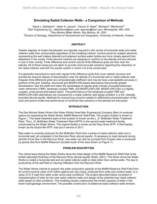
The Des Moines Water Works (the Water Works) hired Barr Engineering Company (Barr) to evaluate
options for expanding the Water Works’ Maffitt Reservoir Well-Field. The project location is shown in
Figure 1. The water treatment plant at this location is known as the L. D. McMullen Water Treatment
Plant. The L. D. McMullen Water Treatment Plant (WTP) is the second water treatment facility
constructed by the Water Works. The original facility is known as the Fleur Drive WTP. A third facility,
known as the Saylorville WTP, was put in service in 2011.
Raw water is currently produced for the McMullen Plant from a series of radial collector wells and a
horizontal well, all completed in the Raccoon River alluvial aquifer. If necessary to meet demand during
periods of low flow in the Raccoon River, raw water can also be pumped from Crystal Lake or produced
by gravity flow from Maffitt Reservoir (located south of the area shown on Figure 1).
PROBLEM DESCRIPTION
The critical issue facing the Water Works since the initial design of the Maffitt Reservoir Well-Field is the
limited saturated thickness of the Raccoon River alluvial aquifer (Rash, 2001). This factor drove the Water
Works to install a horizontal well and six radial collector wells to date rather than vertical wells. The key to
productivity of the well field is inducing infiltration from the Raccoon River.
The Water Works intends to expand raw water production capacity at the Maffitt Reservoir Well-Field from
its current nominal value of 25 million gallons per day (mgd), produced from wells and surface water, to a
value of 37.5 mgd from wells under worst-case conditions. The project described below consisted of
characterization of sites for two new radial collector wells and design of the potential new radial collector
wells based on field conditions. The modeling results underscored the limited capacity of wells in this
harsh hydrogeologic environment. The possible construction of additional radial collector wells remains
MODFLOW and More 2015: Modeling a Complex World - IGWMC - Maxwell, Hill, Zheng & Tonkin
350

2. part of the Water Works’ long term strategy, however, well-field capacity will initially be increased through
a strategy of maximizing the use of surface water from former sand and gravel quarries that have been
converted to lakes. This surface water will supplement the current yield from the existing system of wells.
Modeling Software Selection
As described above, design of radial collector wells requires greater model discretization than is typical
for vertical well field design. Unlike many modeling applications, greater discretization is needed at the
depth of the laterals than near the surface, even in an application with irregularly-shaped surface water
bodies such as shown in Figure 1.
Several methods and groundwater
modeling codes of varying
sophistication have been utilized in
the design of radial collector wells
(Yeh and Chang, 2013). The decision
was made to use MODFLOW-NWT
(Niswonger, et al, 2011) and to
employ the multi-node well package
(MNW; Halford and Hanson, 2002)
based on the code’s open source,
degree of benchmarking,
applicability, and compatibility with
predictive analysis methods (Doherty
and Hunt, 2010).
A regional groundwater flow model
was developed and two highly-
discretized local models (TMRs) were
constructed that were iteratively
coupled with the regional model by
specifying heads for the cells around
the perimeter of each TMR based on
the regional model and by mapping
simulated flows to the radial collector
well on a cell-by-cell basis back to
the regional model using the WEL
package.
The groundwater flow model was
calibrated to measurements taken during site characterization and based on observed well field
performance. The calibration was automated using PEST (Watermark Numerical Computing, 2005) with
pilot point parameterization of hydraulic conductivity and storage parameters. The same aquifer
parameter values were used in the TMR cells as in the parent cells to prevent upscaling issues. The
regional groundwater flow model has 205,470 active cells in two layers and each TMR has 65,522 active
cells, also in two layers. A 5:1 ratio of nested to parent cell plan view dimensions was used.
COMPARISON WITH A MODFLOW-USG APPLICATION
For purposes of comparison with a modeling approach released since the project was completed, the
regional model described above was converted to MODFLOW-USG (Panday, et al, 2013) and a nest with
the same 5:1 ratio of nested to parent cell plan view dimensions was placed at the location of one of the
TMRs. The nested grid penetrates both layers of the parent model. The unstructured grid has 262,846
active cells; the model size would be reduced further by having the nested grid penetrate only the deeper
layer where the radial collector well laterals are simulated. This option of a partially-penetrating area of
greater discretization that does not extend into the top model layer is not an option with the local grid
Figure 1. Project Location (west of Des Moines, Iowa)
MODFLOW and More 2015: Modeling a Complex World - IGWMC - Maxwell, Hill, Zheng & Tonkin
351

3. refinement (LGR) packages (Mehl and Hill, 2007; Mehl and Hill, 2013), but is advantageous for designing
radial collector wells. Rather than the MNW well package, the connected linear network (CLN) package
was used to simulate a radial collector well in the lower layer of the nested grid.
Similarities in the modeling approaches
The lateral configuration that was to be simulated was represented as a polyline shapefile and intersected
with the highly-discretized model grid. The methods presented in Haitjema, et al (2010) were used to
determine the resistance to flow (inverse of leakance) from a given model cell into the length of lateral
crossing the cell.
Differences in the modeling approaches model behavior
The cell-to-well conductance is input to the MNW package whereas the leakance is input to the CLN
package. A limiting head can be specified for the MNW cell below which the simulated head will not be
drawn. Total pumping from the group of MNW cells representing the radial collector will be reduced such
that none of the heads in any of the model cells is below the limiting head specified for that cell. In other
words, the well is drawdown-limited. The CLN package does not have a similar setting. If a drawdown-
limited approach is desired using the CLN package, a CHD cell is specified in one of the CLN cells. The
CLN package allows explicit simulation of the caisson, including storage effects. This offers promise in
simulating performance tests of radial collector wells.
A specified discharge rate is simulated by placing a WEL cell in one of the CLN nodes. Initial results
indicate it is advantageous to explicitly simulate the caisson for discharge-specified wells. Model runs that
did not converge without simulating the caisson converged rapidly when the 2-meter diameter caisson
was simulated. In other applications of the CLN package to vertical wells with specified discharge,
modelers have reported model non-convergence. The large storage capacity of this feature may provide
a “numerical buffer” that dampens large head changes as the code solves for the head distribution in the
CLN. Convergence issues did not occur when simulating drawdown-controlled wells whether or not the
caisson was explicitly simulated.
Performance comparison
The iteratively-coupled model was run until the largest change in head in the perimeter specified heads
cells was less than 0.001 meters, which took 95 seconds. The MODFLOW-USG model ran in 37
seconds. The models included drawdown-controlled wells and the simulated discharges and head
distributions using the two modeling approaches were essentially identical.
Simulating frictional head losses and turbulent flow in the laterals
The official USGS release of MODFLOW-USG assumes laminar flow in the CLNs (Panday, et al, 2013).
The developmental version of MODFLOW-USG includes three solutions for that account for frictional
head losses in the CLNs: Darcy-Weisbach, Hazen-Williams, and Manning’s equations (Panday, 2015).
Darcy-Weisbach and Hazen-Williams also account for turbulent flow in the CLNs. Notes on the
application of these flow solutions to the radial collector well design are presented below.
Manning’s equation. Using a value of Manning’s roughness coefficient considered representative of
wire-wound well screen (n = 0.018, Bakiewicz et al. (1985) in Misstear, 2012) and a units conversion
factor (C) of 86,400 for time units of days, simulated discharge from a drawdown-controlled radial
collector well was reduced from 2.48 to 2.44 mgd. In this case, the CLN input CONDUITK is set to n/C.
Hazen-Williams equation. The Hazen-Williams relative roughness factor (C) typically ranges from 60 for
old pipes in bad condition to 140 for extremely smooth and straight pipes (Streeter and Wylie, 1979), and
the conversion factor (k) for units of meters and days is 73,353.6. In this case, the CLN input CONDUITK
is set to kC. An equivalent discharge to that calculated using Manning’s equation is produced if the
Hazen-Williams relative roughness factor is set to 86.
MODFLOW and More 2015: Modeling a Complex World - IGWMC - Maxwell, Hill, Zheng & Tonkin
352

4. Darcy-Weisbach equation. The Darcy-Weisbach solution yields an equivalent discharge to the other
solutions for water with a kinematic viscosity value of 0.087 m
2
/day (water at 20
o
C, Streeter and Wylie,
1979) and a mean roughness height of 0.0102 m. In this case, the CLN input CONDUITK is set to the
mean roughness height and the GRAVITY and VISCOSITY keywords are input in data set 1.
SUMMARY
MODFLOW-USG and the CLN package are well-suited to provide the high degrees of local discretization
required for the design of radial collector wells. In addition to faster model set-up and solution times, the
non-linear solutions for flow in the developmental version of the CLN package remove the need to
estimate head losses in the lateral using other means. The non-linear solutions for flow in the CLNs will
eventually be added to the official USGS release of MODFLOW-USG, however, the timing of this release
is not known (Panday, 2015).
REFERENCES
Doherty, J.E., and Hunt, R.J., 2010, Approaches to highly parameterized inversion—A guide to using
PEST for groundwater-model calibration: U.S. Geological Survey Scientific Investigations Report
2010–5169, 59 p.
Halford, K.J., and Hanson, R.T., 2002: MODFLOW-2000, User guide for the drawdown-limited, Multi-
Node Well (MNW) Package for the U.S. Geological Survey’s modular three-dimensional ground-
water flow model, Versions MODFLOW-96 and MODFLOW-2000, USGS Open-File Report 02-
294, Reston, Virginia. 33 p.
Haitjema, H., S. Kuzin, V. Kelson and D. Abrams, 2010. Modeling Flow into Horizontal Wells in a Dupuit-
Forchheimer Model. Ground Water, Vol. 48, No. 6, p. 878-883.
Mehl, S.W., and Hill, M.C., 2007. MODFLOW-2005, The U.S. Geological Survey modular ground-water
model—Documentation of the multiple-refined-areas capability of local grid refinement (LGR) and
the boundary flow and head (BFH) package: U.S. Geological Survey Techniques and Methods 6-
A21, 13 p.
Mehl, S.W., and Hill, M.C., 2013, MODFLOW–LGR—Documentation of ghost node local grid refinement
(LGR2) for multiple areas and the boundary flow and head (BFH2) package: U.S. Geological
Survey Techniques and Methods book 6, chap. A44, 43 p.
Misstear, B. (2012). Some key issues in the design of water wells in unconsolidated and fractured rock
aquifers. Italian Journal of Groundwater (2012).
Niswonger, R.G., Panday, S., and Ibaraki, Motomu, 2011. MODFLOW-NWT, A Newton formulation for
MODFLOW-2005: U.S. Geological Survey Techniques and Methods 6-A37, 44 p.
Panday, Sorab, Langevin, C.D., Niswonger, R.G., Ibaraki, Motomu, and Hughes, J.D., 2013, MODFLOW–
USG version 1: An unstructured grid version of MODFLOW for simulating groundwater flow and
tightly coupled processes using a control volume finite-difference formulation: U.S. Geological
Survey Techniques and Methods, book 6, chap. A45, 66 p.
Panday, Sorab, 2015. Personal communication.
Rash, Vernon D., 2001. Predicting Yield and Operating Behavior of a Horizontal Well. AWWA Annual
Conference. Washington, DC.
Streeter, V.L. and E.B. Wylie, 1979. Fluid Mechanics, 7th Edition. McGraw-Hill Book Company, NY, NY.
562 p.
Watermark Numerical Computing, 2010. PEST: Model-Independent Parameter Estimation. User Manual.
5th edition.
Yeh, H.D., and Chang Y.C., 2013. Recent advances in modeling of well hydraulics. Advances in Water
Resources, Vol. 51, p. 27-51.
MODFLOW and More 2015: Modeling a Complex World - IGWMC - Maxwell, Hill, Zheng & Tonkin
353