SlideShare a Scribd company logo
1 of 123
Coursework Project
“Companies are paying out too much in dividends. Shareholders
have too much power in corporate affairs. In addition, company
law should be changed to allow more power for other
“stakeholders” – customers and employees. So says Andy
Haldane, chief economist at the Bank of England, in a critique
that will be seized upon as compelling evidence of broken
capitalism.” Bill Jamieson
The assertion within the above quote is that companies are not
investing for the future as much as they should. Thus, pursuing
short-termism – a focus on immediate gains rather than long-
term prospects. Given this assertion, you are required to:
a) Evaluate dividend policy theories and whether companies
should maximise shareholders wealth or satisfice stakeholders’
other objectives.
(25 marks)
b) Select a company of your choice from the top 250 UK listed
companies for which you can easily access annual reports,
especially information on dividend policy, share prices, and
capital structure for a continuous period of not less than 11
years. Using this information, critically evaluate whether the
firm’s dividend policy have had any impact on its share price.
(35 marks)
c) Using Fisher-Hirshleifer model, examine firms’ investment
decisions, owners’ consumption decisions in relation to the role
of capital markets.
(20 marks)
d) Discuss the importance of merger and acquisition for
developed economy (20 marks
Total marks (100
marks)
Your coursework should not exceed 3000 words. There is no
fixed penalty for exceeding the word count, but students should
be made aware that the marker will not consider any work after
the +10% word count tolerance has been reached, within the
allocation of marks. Students may therefore be penalised for a
failure to be concise and for failing to conclude their work
within the word count specified.
Indicative contents
a)
· Critically review / evaluate dividend policies
· What is the impact of dividend payment on companies’
investment practices and their capital structure?
· Who are stakeholders within a company and what are
competing interests of stakeholders versus shareholders?
(35 marks)
b)
· Role of dividend in terms of signalling theory
· Use data to benchmark comparison between share price and
firm’s dividend policy
· To carry out data analysis and comment what other factors
than dividend pay-out impact on company’s share price
(35 marks)
c)
· Use HL model to explain the operation of the separation
theorem.
· Infer the relationship between capital markets and
consumption decision
· Relate the HL model with agency relationship
(30 marks)
d)
· Define merger and acquisition
· Discuss importance of merger
· Why merger and acquisitions are more active in developed
countries
READING ASSIGNMENT
Your project must be submitted as a Word document (.docx,
.doc)*. Your project will be individually graded by your
instructor and therefore will take up to a few weeks to grade.
Be sure that each of your files contains the following
information:
· Your name
· Your student ID number
· The exam number
· Your email address
To submit your graded project, follow these steps:
· Log in to your student portal.
· Click on Take Exam next to the lesson you’re working on.
· Find the exam number for your project at the top of the Project
Upload page.
· Follow the instructions provided to complete your exam.
Be sure to keep a backup copy of any files you submit to the
school!
This case is based on real financial data provided by a retail
automobile dealership (Motomart) seeking to relocate closer to
an existing retail dealership. You’ll examine the mixed cost
data from Motomart and apply both high-low and regression to
attempt to separate mixed costs into their fixed and variable
components for break-even and contribution margin
computations. You’ll find that the data is flawed because
Motomart was a single observation in a larger database. Don’t
attempt to correct the data (e.g., remove outliers or influential
outliers). You’ll be producing a scatterplot and apply high-low
and regression methods to the extent practicable and writing a
summary report of the findings.
Motomart operates a retail automobile dealership. The
manufacturer of Motomart products, like all automobile
manufacturers, produces forecasts. It has long been an industry
practice to use variable costing-based/break-even analyses as
the foundation for these forecasts, to examine their cost
behavior as it relates to the new retail vehicles sold
(NRVS) cost driver. In preparing this financial information, a
common financial statement format and accounting procedures
manual are provided to each retail auto dealership. The
dealership is required to produce monthly financial statements
using the guidelines provided by this common accounting
procedures manual, and then furnish these financial statements
to the manufacturer. General Motors, Ford, Nissan, and all other
automobile manufacturers employ similar procedures manuals.
The use of a common format facilitates the development of
composite financial statements that can be used to estimate
costs and produce financial forecasts for future or proposed
retail dealership sites (Cataldo and Kruck 1998). Zimmerman
(2003) suggests that as many as 77 percents of manufacturers
divide costs into variable and fixed components and that
managers arrive at these estimates by classifying individual
accounts as being primarily fixed or primarily variable (67).
For this case, you’ll examine mixed costs as defined by the
manufacturer. Using the scatterplot, high-low, and regression
methods, separate these mixed costs into their fixed and
variable components. The data is problematic, and a clear
solution won’t exist. Don’t attempt to correct the data by
removing outliers, but make observations based on any patterns
you observe. The case will expose you to actual data and
require you to summarize your findings, including any
conclusions you’re able to reach and why the financial data
makes it impossible to separate the mixed costs into their fixed
and variable components.
Motomart: A Litigation Support Engagement
The Motomart case evolved from a litigation support
engagement. The lead author of this case was hired to analyze
the data and provide expert testimony. His report and testimony
was made available to the public (for a fee to cover
reproduction costs). A broad description of the relevant points
for the Motomart case follows.
Motomart wanted to move their retail automobile dealership,
blaming their location for declining profits and increasing
losses. They provided financial projections, using variable
costing, to show that after the relocation both Motomart and the
existing dealership would be profitable. They created these
financial projections using a database provided by the
manufacturer, which included all North American retail
automobile dealerships. Motomart was one of the observations
or retail automobile dealerships included in the database used to
create these financial projections. You’ll be examining portions
of Motomart’s historical financial data.
The relocation site was quite close to the existing dealership
(which we’ll refer to as Existing Dealer), and Existing Dealer
felt that, if the relocation was permitted, one or both of the
dealerships would fail to break even and eventually go
bankrupt, leading to poor service, or what the industry refers to
as “orphaned” owners of these automobiles.
Antitrust laws provided Existing Dealer with the means to block
the relocation requested by Motomart, but only if it could prove
that the relocation wasn’t in the best interest of the consuming
public. Generally, the only way to prove this is to prove that
there’s simply not enough business for both retail automobile
dealerships to break even (or generate a reasonable return on
investment, given the risks associated with the industry). Again,
the manufacturer, in support of the proposed Motomart
relocation, supplied financial projections showing that both
retail automobile dealerships would be profitable after the
relocation.
The expert witness hired to investigate the merits of the
relocation was given the Motomart data, but not the entire
database that included the Motomart data. The Motomart data
was in such poor form that it wasn’t possible to produce a
financial forecast. An alternative forecast, not included in this
case, was produced. This alternative forecast did not support the
relocation of Motomart to a site closer to Existing Dealer. The
alternative forecast showed that the market simply couldn’t
support two retail automobile dealerships. The implication was
that, as the weaker of the two dealerships, Motomart was losing
business to Existing Dealer. In conclusion, the relocation
request by Motomart was denied.
Income and Expense Data
The following tables give you information such as income
statements, semi-fixed expenses, and salaries for Motomart.
Look for unusual entries or discrepancies in their records and,
where you can, note the cause of the problems.
Table 3 summarizes financial and cost driver information
produced by Motomart, where new retail vehicles sold (NRVS)
is the cost driver. The account classification method has
resulted in three cost behavior classifications: variable, semi -
fixed, and fixed costs. Semi-fixed is the automobile industry-
specific term used for mixed costs. We’ll assume that
Motomart’s classifications of variable costs (VCs) and fixed
costs (FCs) are correct, and focus our analysis on Motomart’s
semi-fixed or mixed costs.
Table 2
SElECTED HISTORICAl INCOME STATEMENT AND
RElATED MEASURES
1984
1985
1986
1987
1988
Net Variable Revenues*
2,885,969
3,828,255
4,086,667
3,940,799
4,298,748
Semi-Fixed (S-F) Expenses:
Salaries
613,006
968,789
1,211,464
1,289,758
1,360,489
Vacation
600
26,705
19,468
19,059
18,268
Advertising & Training
210,226
288,347
281,219
309,608
371,314
Supplies/Tools/Laundry
31,473
46,141
75,468
65,935
81,252
Freight
5,719
5,987
6,528
5,731
4,663
Vehicle
22,913
23,718
23,664
20,370
19,483
Demonstrators
10,465
4,969
-1,513
4,192
707
Floor-Planning
278,531
301,113
276,201
156,129
305,044
Total S-F Expenses
1,172,933
1,665,769
1,892,499
1,870,782
2,161,220
Fixed Expenses:
Total Fixed Expenses
1,449,208
2,050,172
2,290,867
2,164,362
2,653,620
Operating Profit/(Loss)**
263,828
112,314
-96,699
-94,345
-516,092
New Retail Vehicles Sold
1,798
1,977
1,674
1,450
1,897
Notes:
* Revenues less variable costs equal Net Variable Revenues (or
Contribution Margin, in aggregate).
** Net Variable Revenue less Total S-F Expenses less Total
Fixed Expenses equals Operating Profit/(Loss).
Table 3 provides five years of monthly data (N=60) for NRVS
and the related semi-fixed or mixed cost measures. Semifixed
costs were significant. Recall that they ranged from nearly $1.2
million for calendar and fiscal year (FY) 1984 to almost $2.2
million for FY 1988 (see Table 2).
Table 3
SEMI-FIXED (MIXED) EXPENSES FOR THE 60-MONTH
PERIOD (FY 1984 THROUGH 1988)
Mo
NRVS
Salary
Vacation
Adv/Trng
SplyTls/Lndry
1
197
$ 52,951
$ -
$ 22,561
$ 1,118
2
133
$ 47,054
$ -
$ 19,040
$ 3,573
3
132
$ 55,372
$ -
$ 14,373
$ 1,388
4
141
$ 46,114
$ -
$ 15,022
$ 2,894
5
182
$ 48,309
$ -
$ 19,966
$ 1,896
6
156
$ 49,643
$ -
$ 12,019
$ 1,188
7
196
$ 55,784
$ 300
$ 13,217
$ 3,912
8
178
$ 47,957
$ -
$ 17,303
$ 2,012
9
159
$ 53,743
$ -
$ 16,535
$ 2,717
10
141
$ 53,109
$ -
$ 23,821
$ 1,102
11
152
$ 45,491
$ 300
$ 14,146
$ 2,630
12
31
$ 57,479
$ -
$ 22,223
$ 7,043
13
280
$ 49,049
$ -
$ 19,992
$ 1,999
14
136
$ 46,698
$ 300
$ 20,251
$ 1,192
15
174
$ 59,790
$ 200
$ 20,082
$ 1,336
16
171
$ 80,773
$ 600
$ 26,716
$ 3,873
17
167
$ 71,130
$ 9,212
$ 25,223
$ 5,560
18
161
$ 82,490
$ 6,007
$ 21,106
$ 1,737
19
173
$ 98,172
$ 500
$ 17,799
$ 1,847
20
161
$ 90,685
$ 2,690
$ 28,038
$ 4,415
21
167
$ 97,771
$ 600
$ 37,284
$ 2,827
22
153
$ 87,129
$ 1,740
$ 24,236
$ 5,836
23
201
$ 95,910
$ 2,074
$ 27,244
$ 3,387
24
33
$ 09,192
$ 2,782
$ 20,376
$ 12,132
25
227
$ 89,041
$ 1,880
$ 26,719
$ 4,383
26
150
$ 92,165
$ 3,602
$ 14,727
$ 10,231
27
142
$ 88,981
$ 744
$ 27,880
$ 7,734
28
104
$ 95,898
$ 960
$ 21,872
$ (684)
29
121
$ 96,245
$ -
$ 18,705
$ 8,329
30
99
$ 106,364
$ -
$ 23,835
$ 2,540
31
150
$ 90,564
$ 1,950
$ 25,605
$ 5,862
32
144
$ 98,418
$ 1,540
$ 17,763
$ 6,998
33
154
$ 110,436
$ 2,693
32,379
$ 8,131
34
130
$ 102,042
$ 1,060
$ 19,324
$ 6,026
35
202
$ 124,413
$ 3,519
$ 22,412
$ 9,120
36
51
$ 116,897
$ 1,520
$ 29,998
$ 6,798
37
148
$ 97,083
$ 1,080
$ 9,112
$ 6,627
38
153
$ 104,727
$ 3,230
$ 38,616
$ 5,892
39
83
$ 95,622
$ 953
$ 22,690
$ 3,450
40
101
$ 96,438
$ 1,244
$ 14,703
$ 5,259
41
140
$ 114,995
$ -
$ 28,764
$ 2,294
42
132
$ 105,337
$ 160
$ 27,253
$ 8,155
43
112
$ 98,989
$ 2,480
$ 24,419
$ 1,621
44
127
$ 124,352
$ 1,800
$ 26,011
$ 902
45
139
$ 115,875
$ 1,417
$ 24,492
$ 5,158
46
156
$ 113,035
$ 1,820
$ 31,158
$ 2,901
47
126
$ 119,106
$ 3,338
$ 32,213
$ 14,426
48
33
$ 104,199
$ 1,537
$ 30,177
$ 9,250
49
209
$ 98,938
$ 1,866
$ 26,737
$ 1,694
50
124
$ 108,606
$ 3,676
$ 31,084
$ 9,040
51
131
$ 106,396
$ 1,197
$ 33,278
$ 2,099
52
144
$ 106,778
$ 241
$ 32,657
$ 9,328
53
93
$ 124,805
$ 500
$ 29,794
$ 4,268
54
199
$ 110,153
$ 1,910
$ 38,431
$ 5,407
55
170
$ 117,276
$ 800
$ 27,640
$ 9,305
56
186
$ 112,055
$ 980
$ 28,657
$ 1,803
57
200
$ 114,765
$ 1,695
$ 36,425
$ 8,839
58
146
$ 128,007
$ 1,560
$ 27,720
$ 10,944
59
222
$ 116,811
$ 2,249
$ 27,941
$ 5,775
60
73
$ 115,899
$ 1,594
$ 30,950
$ 30,950
Table 3 Continued
SEMI-FIXED (MIXED) EXPENSES FOR THE 60-MONTH
PERIOD (FY 1984 THROUGH 1988)
Mo
Freight
Vehicles
Demo's
Floor-Plan
Total
1
$ 382
$ 2,052
$ 1,881
$ (78,173)
$ 2,772
2
$ 409
$ 1,405
$ 695
$ 28,456
$ 100,632
3
$ 742
$ 1,380
$ 469
$ 34,423
$ 108,147
4
$ 675
$ 2,057
$ 125
$ 5,697
$ 72,584
5
$ 572
$ 1,603
$ 131
$ 34,599
$ 107,076
6
$ 407
$ 2,524
$ 1,229
$ 53,737
$ 120,747
7
$ 643
$ 2,348
$ 1,206
$ 5,507
$ 82,917
8
$ 605
$ 1,208
$ 436
$ 32,436
$ 101,957
9
$ 209
$ 2,400
$ 1,476
$ 28,950
$ 106,030
10
$ 184
$ 2,076
$ 1,168
$ 20,876
$ 102,336
11
$ 331
$ 1,677
$ 635
$ 45,278
$ 110,488
12
$ 560
$ 2,183
$ 1,014
$ 66,745
$ 157,247
13
$ 582
$ 1,927
$ (477)
$ (30,104)
$ 42,968
14
$ 603
$ 1,156
$ 1,839
$ 50,583
$ 122,622
15
$ 492
$ 1,898
$ 1,260
$ 18,803
$ 103,861
16
$ 559
$ 1,808
$ 510
$ 23,080
$ 137,919
17
$ 356
$ 1,816
$ 2,350
$ 18,774
$ 134,421
18
$ 439
$ 1,384
$ (288)
$ 23,802
$ 136,677
19
$ 1,628
$ 1,962
$ 1,591
$ 33,848
$ 157,347
20
$ (12)
$ 2,446
$ (3,308)
$ 13,480
$ 138,434
21
$ 480
$ 2,296
$ 1,709
$ 22,965
$ 165,932
22
$ 79
$ 3,175
$ 798
$ 18,898
$ 141,891
23
$ 188
$ 1,287
$ (2,025)
$ 38,699
$ 166,764
24
$ 593
$ 2,563
$ 1,010
$ 68,285
$ 216,933
25
$ 769
$ 2,205
$ 2,493
$ (44,140)
$ 83,350
26
$ 593
$ 2,289
$ (2,051)
$ 36,311
$ 157,867
27
$ 414
$ 1,891
$ 386
$ 19,865
$ 147,895
28
$ 425
$ 2,288
$ 178
$ 19,013
$ 139,950
29
$ 483
$ 2,223
$ (262)
$ 16,228
$ 141,951
30
$ 417
$ 1,683
$ (1,356)
$ 37,637
$ 171,120
31
$ 222
$ 1,586
$ 486
$ (1,121)
$ 125,154
32
$ 49
$ 1,751
$ (1,924)
$ 34,757
$ 159,352
33
$ 818
$ 2,082
$ 1,547
$ 26,419
$ 184,505
34
$ 1,015
$ 1,714
$ 132
$ 21,134
$ 52,447
35
$ 1,255
$ 2,173
$ (2,337)
$ 18,578
$ 179,133
36
$ 68
$ 1,779
$ 1,195
$ 91,520
$ 249,775
37
$ 565
$ 1,324
$ 1,164
$ (73,753)
$ 43,202
38
$ 369
$ 1,523
$ (1,839)
$ 30,443
$ 182,961
39
$ (182)
$ 2,087
$ 454
$ 17,725
$ 142,799
40
$ 709
$ 2,095
$ 868
$ 26,402
$ 147,718
41
$ 1,006
$ 1,304
$ (1,990)
$ (3,789
$ 142,584
42
$ 521
$ 1,667
$ 1,869
$ 15,090
$ 160,052
43
$ 514
$ 1,040
$ 329
$ (945)
$ 128,447
44
$ 917
$ 2,880
$ (1,897)
$ 30,405
$ 185,370
45
$ (77
$ 1,281
$ 2,959
$ 14,781
$ 165,886
46
$ 450
$ 2,259
$ 417
$ 15,613
$ 167,653
47
$ 120
$ 1,394
$ (2,659)
$ 40,968
$ 208,906
48
$ 819
$ 1,516
$ 4,517
$ 43,189
$ 195,204
49
$ 853
$ 1,657
$ 601
$ (20,127)
$ 112,219
50
$ 498
$ 2,266
$ (284)
$ 18,236
$ 173,122
51
$ 605
$ 1,952
$ 668
$ 15,176
$ 161,371
52
$ 483
$ 1,852
$ 1,409
$ 25,245
$ 177,993
53
$ 788
$ 1,704
$ (1,771)
$ 6,493
$ 166,581
54
$ 529
$ 1,882
$ 453
$ 21,851
$ 180,616
55
$ (180)
$ 977
$ 1,310
$ 7
$ 157,135
56
$ 242)
$ 846
$ (2,844)
$ 17,192
$ 158,447
57
$ 859
$ 2,856
$ 1,532
$ 14,864
$ 181,835
58
$ (492)
$ 1,864
$ 1,400
$ 10,121
$ 181,124
59
$ 245
$ 1,141
$ (3,513)
$ 7,946
$ 158,595
60
$ 717
$ 486
$ 1,746
$ 188,040
$ 352,182
Recall the cost function applying to the high-low and regression
methods, which are provided in a variety of forms, depending
on the texts you used in your previous math, economics, or
accounting courses. Below is a brief outline of the high-low and
regression methods.
For the high-low method to work, the $H and #H and the $L and
#L measures must be from the same accounting period.
Preparing Graphs
The single cost driver and nonfinancial measure in Table 3 is
new retail vehicles sold (NRVS or X in the above cost
function). There are eight financial measures (salary; vacation;
advertising and training; supplies, tools, and laundry; freight;
vehicles; demonstrators; and floor-planning [also known in the
automobile retail industry as interest expense relating to new
car inventory]), as well as a total (aggregate measure) provided
for all eight financial measures (or the Y in the above cost
function).
Using NRVS, the only available cost-driver, use Excel to
prepare nine separate scatter plots and cost function-based trend
lines and nine separate line graphs for each of the financial
measures provided in Table 3. The images below are an example
of completed graphs for salaries.
A Scatterplot Graph for Motomart SalariesA Line Graph for
Motomart Salaries
Now examine, on a preliminary basis, the pattern or trend (or
lack thereof) for each of the “X” (NRVS) and “Y” (financial
measure) data pairs and consider the following questions:
· You’re observing these data pairs for a 60-month period (i.e.,
five years); are any annual or other seasonal patterns or trends
immediately apparent?
· Do the slopes of the trend lines (i.e., variable costs) make
sense?
In the case of salaries (see the graphs above), there’s no
apparent trend or pattern. It’s odd that salaries decrease as
NRVS increases—in fact, this doesn’t make any sense.
However, it’s consistent with the high-low results, which also
didn’t make sense. But remember, since this data came from
Motomart, the firm attempting to relocate, it’s real and from an
actual litigation support engagement (not a textbook problem),
so it won’t necessarily work out perfectly.
The cost equation in Table 4 shows fixed costs (FC) at
$106,866.00 and variable costs to be used to “reduce” total
costs (TC) by $110.10 per NRVS. Compare the salary figures
and coefficients (in bold type) to the scatterplot graph for
Motomart Salaries. Notice that if you extended the trend line in
Figure 4, it would hit the y-axis intercept at $106,866.00 (the
fixed cost). Also, notice that the R-squared (R-sq) measure in
Table 4 equals 4.1 percent.
Table 4
SALARY = $106,866.00 – $110.10 NRVS
Predictor
Coefficient
Std Deviation
t-statistic
p-value
Constant
106,866.00
10,793.00
9.90
0.000
NRVS
110.10
70.17
–1.57
0.122
s = 25300 r-sq = 4.1%
Analysis of Variance
SOURCE
DF
SS
MS
F-statistic
p-value
Regression
1
261,795
261,795
0.10
0.754
Error
58
152,801,120
2,634,502
Total
59
153,062,912
Your math and statistics courses probably reviewed the use of
the t-statistic, overall F-statistic, and related p-values, as well
as some of the other measures presented here. Our application is
a very simple one, so we’ll focus on only the R-squared
measure. The other measures are provided in this example only
for completeness.
Because the high-low technique didn’t work, it makes sense that
the regression technique wouldn’t work well, either. Therefore,
the results for high-low and regression are consistent. The
advantage of the regression technique is that it mathematically
quantifies the level of the problem or difficulty with the data. In
this case, one of simple regression, the R-squared measure tells
the story. Still focusing on the salaries example in Figure 5, the
R-squared measure tells us that only 4.1 percent of the total or
mixed or semi-fixed cost is explained by NRVS. This means
that that cost equation developed from this historical data isn’t
helpful in predicting future costs, as nearly 96 percent of the
cost behavior, through use of this equation, remains
unexplained.
Requirements
The project requires five steps to be presented.
Step 1 – Provide comments on a 5-year Income Statement.
Step 2 – Discuss patterns in expense items.
Step 3 – Identify High/Low activity levels.
Step 4 – Compute cost equations.
Step 5 – Summarize your findings.
In one Word document, provide individual sections for each
Step. This Word document along with the Excel file (described
below) will be uploaded when you click on the Take Exam
button on your Student Portal to submit your project (described
under “Submitting Your Assignment” later in the instructions).
This Senior Capstone project highlights your knowledge and the
skills you have developed over the course of your education.
There is nothing “new” to be learned here.
The knowledge and skills required for this project include
English Composition, Financial Accounting, Managerial
Accounting, Business Statistics and the abilities to think
critically and to present your work in a professional manner.
If you are unsure or don’t understand something about the
project, then go back to your previous subjects to review. For
example, if you don’t remember how to use the High/Low
Method, the revisit your Managerial Accounting to refresh your
memory on how to use the High/Low Method
Remember, there is nothing “new” here. Everything about this
project you should already know how to do.
At the beginning of the assignment, on the right-hand side under
"Optional Study Materials" select the "PPMC Excel
Spreadsheet" menu item to download the required Excel
spreadsheet.
· The Excel file provides a detailed example of what needs to be
done for one of the expenses in order to fill out the figures
required in Steps 3 & 4. You will include this Excel file as part
of your project submission along with the Word document you
create to present this project.
· There is a “60 Months” worksheet that has the 60 months of
data already entered. There is also a “Sample” worksheet that an
example of how to calculate the R-sq.
· There is a “PLOT – SALARY” worksheet that shows how the
FC, VC and R-sq figures are calculated for Salary.
· There is also a “high&low” worksheet for help with the
high/low method in Step 3.
· Complete and include the Excel spreadsheet. You will need to
create new worksheets for each of the other expenses following
the example to calculate the figures needed for Table 5.
Operating Profits and Semi-Fixed Expenses
Step 1
First, using Tables 2–4, note the pattern of operating profits (or
losses) over the five-year period. Then focus only on the semi-
fixed expenses contained in Table 2. Do any amounts appear to
be odd? (Think about whether the figures are right or wrong.
What is it about the individual numbers that is not “right”?)
Next, briefly comment on the five-year pattern or trend for
operating profit/loss measures. You should be able to respond to
this step in a few well-written sentences.
Step 2
Focus only on the detailed semi-fixed expense contained in
Table 3. Are there any unusual or odd patterns you might note
in this detailed financial data? There are 5 expenses that have
an oddity about them which doesn’t make sense. Similar to Step
1, what is it about the individual numbers that are not “right”?
There are 4 expenses that “stick out” as not being correct and
one that has an unusual pattern. attention. You should be able to
respond to this requirement in a few well-written sentences.
Briefly comment on only the most obvious or apparent measures
or patterns, by expense item.
Step 3
Identify the high and low measures in each column, just as you
would in preparation for the application of the high-low method
or technique. For example, in Table 3 the high measure for the
cost driver (NRVS) is 280 NRVS in month 13 and the low
measure is 31 NRVS in month 12. Repeat this process for each
of the eight separate semi-fixed expense columns and also for
the total expense column. Insert a table for Step 3 to present
your findings. The table should have three columns;
1. Expense
2. High Figure
3. Low Figure
After the high and low measures have been identified in each
column, try to match each expense column’s high and low
measure, separately, to the highs and lows identified in the
NRVS column. They won’t match. Don’t try to correct the data,
but comment on the potential for application of the high-low
technique. What happens when the high and low activity level
doesn’t match the high and low expense measure? Does this
prevent you from correctly applying the high-low technique?
Don’t overanalyze this data, because there’s a problem with it
and you don’t have sufficient information to correct it. Merely
summarize your observations and unsuccessful attempts to
match the high and low NRVS months (identified above),
separately, with each of the high and low expense measure
months. You should be able to do this in a very few well-written
sentences.
Step 4
Using the Excel file "Exam 500896 - Motomart Excel
Spreadsheet" as per the instructions found above under the
"Project Requirements", reproduce and complete the following
Table 5 and answer the four questions. The Excel file provides
an example of how to arrive at the figures that need to be
entered into the Table. You will create new worksheets for each
of the remaining expenses. Do the work to arrive at the figures
for each expense. Be sure to include the Excel file as part of
your submission to "backup" the data presented in the Table in
the Word document being submitted.
The Excel spreadsheet, while it will be included in your
submission for the project, will not be graded. It is supporting
documentation for what is being presented in the Word
document. Only the information that is in the Word document
will be graded.
The FC and VC should be rounded to the nearest dollar. The R-
sq is a percentage figure carried out to 2 decimal places.
Table 5
Column
Expense
FC
VC
R-sq
1
Salaries
$106,866
–$110
4.10%
2
Vacation
3
Advertising and training
4
Supplies/tools/laundry
5
Freight
6
Vehicles
7
Demonstrators
8
Floor planning
Computed total
9
Total
Complete the cost equations for the table. Use the R-squared as
the single measure of “goodness of fit.” Don’t attempt to
improve your results with the elimination of “outliers” or
“influential outliers.” As you complete Table 5, answer the
following questions:
1. What problems did you encounter?
2. Are the R-squared measures high or low?
3. Are the slopes negative or positive?
4. Are your conclusions consistent with those from the high-low
effort?
Step 5
Summarize your findings by answering the following questions:
1. Can the Motomart data be used to prepare a reliable financial
forecast? Why or why not?
2. If Motomart is included in the very large database used to
prepare the financial forecast that supports the relocation of
Motomart closer to Existing Dealer, what concerns might
present themselves with respect to the remainder of the database
used for this forecast?
3. Would you rely on this forecast?
Writing Guidelines
Refer to the “Submitting Your Work” section at the end of this
book for details on submission requirements for the Motomart
Case assignment.
Grading Criteria
Your assignment will be evaluated according to the following
criteria:
Content
80 percent
Written Communication
10 percent
Format
10 percent
Criteria
Grade
Content 80 pts
· Step 1 – Provides comments on 5-year income statement
(worth 10 points)
· Step 2 – Discuss patterns in expense items (worth 10 points)
· Step 3 – Identify high and low activity levels (worth 10
points)
· Step 4 – Compute cost equations (worth 30 points)
· Step 5 – Summarize your findings (worth 20 points)
Written Communication 10 pts
· Answers each question in complete sentences leading to well -
structured responses to each Step listed above.
· Uses correct grammar, spelling, punctuation, and sentence
structure
· Provides clear organization by using words like first, however,
on the other hand, and so on, consequently, since,
next, and when
· Makes sure the paper contains no typographical errors
Format 10 pts The paper is double-spaced, typed in font size 12.
It includes the student’s
· Name and address
· Student number, Course title and number, and project number
Total Grade
%
Submitting Your Work
Writing Guidelines
1. Type your submission, double-spaced, in a standard print
font, size 12. Use a standard document format with 1-inch
margins. (Do not use any fancy or cursive fonts.)
2. Include the following information at the top of your paper:
a. Name and complete mailing address
b. Student number
c. Course title and number (Senior Capstone: Business, BUS
450)
d. Project number (see Format instructions)
e. Project title (Professional Development Activity, Case 1,
etc.)
3. Read the assignments carefully and complete each one in the
order given.
4. Be specific. Limit your submission to the questions asked and
issues mentioned.
5. If you include quotes or ideas from textbooks or other
sources, provide a reference page in either APA or MLA style.
On this page, list books, Web sites, journals, or any other
references used in preparing the paper.
6. Proofread your work carefully. Check for correct spelling,
grammar, punctuation, and capitalization.
NOTES
Top of Form
Bottom of Form
READING ASSIGNMENT
Your project must be submitted as a Word document (.docx,
.doc)*. Your project will be individually graded by your
instructor and therefore will take up to a few weeks to grade.
Be sure that each of your files contains the following
information:
· Your name
· Your student ID number
· The exam number
· Your email address
To submit your graded project, follow these steps:
· Log in to your student portal.
· Click on Take Exam next to the lesson you’re working on.
· Find the exam number for your project at the top of the Project
Upload page.
· Follow the instructions provided to complete your exam.
Be sure to keep a backup copy of any files you submit to the
school!
This case is based on real financial data provided by a retail
automobile dealership (Motomart) seeking to relocate closer to
an existing retail dealership. You’ll examine the mixed cost
data from Motomart and apply both high-low and regression to
attempt to separate mixed costs into their fixed and variable
components for break-even and contribution margin
computations. You’ll find that the data is flawed because
Motomart was a single observation in a larger database. Don’t
attempt to correct the data (e.g., remove outliers or influential
outliers). You’ll be producing a scatterplot and apply high-low
and regression methods to the extent practicable and writing a
summary report of the findings.
Motomart operates a retail automobile dealership. The
manufacturer of Motomart products, like all automobile
manufacturers, produces forecasts. It has long been an industry
practice to use variable costing-based/break-even analyses as
the foundation for these forecasts, to examine their cost
behavior as it relates to the new retail vehicles sold
(NRVS) cost driver. In preparing this financial information, a
common financial statement format and accounting procedures
manual are provided to each retail auto dealership. The
dealership is required to produce monthly financial statements
using the guidelines provided by this common accounting
procedures manual, and then furnish these financial statements
to the manufacturer. General Motors, Ford, Nissan, and all other
automobile manufacturers employ similar procedures manuals.
The use of a common format facilitates the development of
composite financial statements that can be used to estimate
costs and produce financial forecasts for future or proposed
retail dealership sites (Cataldo and Kruck 1998). Zimmerman
(2003) suggests that as many as 77 percents of manufacturers
divide costs into variable and fixed components and that
managers arrive at these estimates by classifying individual
accounts as being primarily fixed or primarily variable (67).
For this case, you’ll examine mixed costs as defined by the
manufacturer. Using the scatterplot, high-low, and regression
methods, separate these mixed costs into their fixed and
variable components. The data is problematic, and a clear
solution won’t exist. Don’t attempt to correct the data by
removing outliers, but make observations based on any patterns
you observe. The case will expose you to actual data and
require you to summarize your findings, including any
conclusions you’re able to reach and why the financial data
makes it impossible to separate the mixed costs into their fixed
and variable components.
Motomart: A Litigation Support Engagement
The Motomart case evolved from a litigation support
engagement. The lead author of this case was hired to analyze
the data and provide expert testimony. His report and testimony
was made available to the public (for a fee to cover
reproduction costs). A broad description of the relevant points
for the Motomart case follows.
Motomart wanted to move their retail automobile dealership,
blaming their location for declining profits and increasing
losses. They provided financial projections, using variable
costing, to show that after the relocation both Motomart and the
existing dealership would be profitable. They created these
financial projections using a database provided by the
manufacturer, which included all North American retail
automobile dealerships. Motomart was one of the observations
or retail automobile dealerships included in the database used to
create these financial projections. You’ll be examining portions
of Motomart’s historical financial data.
The relocation site was quite close to the existing dealership
(which we’ll refer to as Existing Dealer), and Existing Dealer
felt that, if the relocation was permitted, one or both of the
dealerships would fail to break even and eventually go
bankrupt, leading to poor service, or what the industry refers to
as “orphaned” owners of these automobiles.
Antitrust laws provided Existing Dealer with the means to block
the relocation requested by Motomart, but only if it could prove
that the relocation wasn’t in the best interest of the consuming
public. Generally, the only way to prove this is to prove that
there’s simply not enough business for both retail automobile
dealerships to break even (or generate a reasonable return on
investment, given the risks associated with the industry). Again,
the manufacturer, in support of the proposed Motomart
relocation, supplied financial projections showing that both
retail automobile dealerships would be profitable after the
relocation.
The expert witness hired to investigate the merits of the
relocation was given the Motomart data, but not the entire
database that included the Motomart data. The Motomart data
was in such poor form that it wasn’t possible to produce a
financial forecast. An alternative forecast, not included in this
case, was produced. This alternative forecast did not support the
relocation of Motomart to a site closer to Existing Dealer. The
alternative forecast showed that the market simply couldn’t
support two retail automobile dealerships. The implication was
that, as the weaker of the two dealerships, Motomart was losing
business to Existing Dealer. In conclusion, the relocation
request by Motomart was denied.
Income and Expense Data
The following tables give you information such as income
statements, semi-fixed expenses, and salaries for Motomart.
Look for unusual entries or discrepancies in their records and,
where you can, note the cause of the problems.
Table 3 summarizes financial and cost driver information
produced by Motomart, where new retail vehicles sold (NRVS)
is the cost driver. The account classification method has
resulted in three cost behavior classifications: variable, semi-
fixed, and fixed costs. Semi-fixed is the automobile industry-
specific term used for mixed costs. We’ll assume that
Motomart’s classifications of variable costs (VCs) and fixed
costs (FCs) are correct, and focus our analysis on Motomart’s
semi-fixed or mixed costs.
Table 2
SElECTED HISTORICAl INCOME STATEMENT AND
RElATED MEASURES
1984
1985
1986
1987
1988
Net Variable Revenues*
2,885,969
3,828,255
4,086,667
3,940,799
4,298,748
Semi-Fixed (S-F) Expenses:
Salaries
613,006
968,789
1,211,464
1,289,758
1,360,489
Vacation
600
26,705
19,468
19,059
18,268
Advertising & Training
210,226
288,347
281,219
309,608
371,314
Supplies/Tools/Laundry
31,473
46,141
75,468
65,935
81,252
Freight
5,719
5,987
6,528
5,731
4,663
Vehicle
22,913
23,718
23,664
20,370
19,483
Demonstrators
10,465
4,969
-1,513
4,192
707
Floor-Planning
278,531
301,113
276,201
156,129
305,044
Total S-F Expenses
1,172,933
1,665,769
1,892,499
1,870,782
2,161,220
Fixed Expenses:
Total Fixed Expenses
1,449,208
2,050,172
2,290,867
2,164,362
2,653,620
Operating Profit/(Loss)**
263,828
112,314
-96,699
-94,345
-516,092
New Retail Vehicles Sold
1,798
1,977
1,674
1,450
1,897
Notes:
* Revenues less variable costs equal Net Variable Revenues (or
Contribution Margin, in aggregate).
** Net Variable Revenue less Total S-F Expenses less Total
Fixed Expenses equals Operating Profit/(Loss).
Table 3 provides five years of monthly data (N=60) for NRVS
and the related semi-fixed or mixed cost measures. Semifixed
costs were significant. Recall that they ranged from nearly $1.2
million for calendar and fiscal year (FY) 1984 to almost $2.2
million for FY 1988 (see Table 2).
Table 3
SEMI-FIXED (MIXED) EXPENSES FOR THE 60-MONTH
PERIOD (FY 1984 THROUGH 1988)
Mo
NRVS
Salary
Vacation
Adv/Trng
SplyTls/Lndry
1
197
$ 52,951
$ -
$ 22,561
$ 1,118
2
133
$ 47,054
$ -
$ 19,040
$ 3,573
3
132
$ 55,372
$ -
$ 14,373
$ 1,388
4
141
$ 46,114
$ -
$ 15,022
$ 2,894
5
182
$ 48,309
$ -
$ 19,966
$ 1,896
6
156
$ 49,643
$ -
$ 12,019
$ 1,188
7
196
$ 55,784
$ 300
$ 13,217
$ 3,912
8
178
$ 47,957
$ -
$ 17,303
$ 2,012
9
159
$ 53,743
$ -
$ 16,535
$ 2,717
10
141
$ 53,109
$ -
$ 23,821
$ 1,102
11
152
$ 45,491
$ 300
$ 14,146
$ 2,630
12
31
$ 57,479
$ -
$ 22,223
$ 7,043
13
280
$ 49,049
$ -
$ 19,992
$ 1,999
14
136
$ 46,698
$ 300
$ 20,251
$ 1,192
15
174
$ 59,790
$ 200
$ 20,082
$ 1,336
16
171
$ 80,773
$ 600
$ 26,716
$ 3,873
17
167
$ 71,130
$ 9,212
$ 25,223
$ 5,560
18
161
$ 82,490
$ 6,007
$ 21,106
$ 1,737
19
173
$ 98,172
$ 500
$ 17,799
$ 1,847
20
161
$ 90,685
$ 2,690
$ 28,038
$ 4,415
21
167
$ 97,771
$ 600
$ 37,284
$ 2,827
22
153
$ 87,129
$ 1,740
$ 24,236
$ 5,836
23
201
$ 95,910
$ 2,074
$ 27,244
$ 3,387
24
33
$ 09,192
$ 2,782
$ 20,376
$ 12,132
25
227
$ 89,041
$ 1,880
$ 26,719
$ 4,383
26
150
$ 92,165
$ 3,602
$ 14,727
$ 10,231
27
142
$ 88,981
$ 744
$ 27,880
$ 7,734
28
104
$ 95,898
$ 960
$ 21,872
$ (684)
29
121
$ 96,245
$ -
$ 18,705
$ 8,329
30
99
$ 106,364
$ -
$ 23,835
$ 2,540
31
150
$ 90,564
$ 1,950
$ 25,605
$ 5,862
32
144
$ 98,418
$ 1,540
$ 17,763
$ 6,998
33
154
$ 110,436
$ 2,693
32,379
$ 8,131
34
130
$ 102,042
$ 1,060
$ 19,324
$ 6,026
35
202
$ 124,413
$ 3,519
$ 22,412
$ 9,120
36
51
$ 116,897
$ 1,520
$ 29,998
$ 6,798
37
148
$ 97,083
$ 1,080
$ 9,112
$ 6,627
38
153
$ 104,727
$ 3,230
$ 38,616
$ 5,892
39
83
$ 95,622
$ 953
$ 22,690
$ 3,450
40
101
$ 96,438
$ 1,244
$ 14,703
$ 5,259
41
140
$ 114,995
$ -
$ 28,764
$ 2,294
42
132
$ 105,337
$ 160
$ 27,253
$ 8,155
43
112
$ 98,989
$ 2,480
$ 24,419
$ 1,621
44
127
$ 124,352
$ 1,800
$ 26,011
$ 902
45
139
$ 115,875
$ 1,417
$ 24,492
$ 5,158
46
156
$ 113,035
$ 1,820
$ 31,158
$ 2,901
47
126
$ 119,106
$ 3,338
$ 32,213
$ 14,426
48
33
$ 104,199
$ 1,537
$ 30,177
$ 9,250
49
209
$ 98,938
$ 1,866
$ 26,737
$ 1,694
50
124
$ 108,606
$ 3,676
$ 31,084
$ 9,040
51
131
$ 106,396
$ 1,197
$ 33,278
$ 2,099
52
144
$ 106,778
$ 241
$ 32,657
$ 9,328
53
93
$ 124,805
$ 500
$ 29,794
$ 4,268
54
199
$ 110,153
$ 1,910
$ 38,431
$ 5,407
55
170
$ 117,276
$ 800
$ 27,640
$ 9,305
56
186
$ 112,055
$ 980
$ 28,657
$ 1,803
57
200
$ 114,765
$ 1,695
$ 36,425
$ 8,839
58
146
$ 128,007
$ 1,560
$ 27,720
$ 10,944
59
222
$ 116,811
$ 2,249
$ 27,941
$ 5,775
60
73
$ 115,899
$ 1,594
$ 30,950
$ 30,950
Table 3 Continued
SEMI-FIXED (MIXED) EXPENSES FOR THE 60-MONTH
PERIOD (FY 1984 THROUGH 1988)
Mo
Freight
Vehicles
Demo's
Floor-Plan
Total
1
$ 382
$ 2,052
$ 1,881
$ (78,173)
$ 2,772
2
$ 409
$ 1,405
$ 695
$ 28,456
$ 100,632
3
$ 742
$ 1,380
$ 469
$ 34,423
$ 108,147
4
$ 675
$ 2,057
$ 125
$ 5,697
$ 72,584
5
$ 572
$ 1,603
$ 131
$ 34,599
$ 107,076
6
$ 407
$ 2,524
$ 1,229
$ 53,737
$ 120,747
7
$ 643
$ 2,348
$ 1,206
$ 5,507
$ 82,917
8
$ 605
$ 1,208
$ 436
$ 32,436
$ 101,957
9
$ 209
$ 2,400
$ 1,476
$ 28,950
$ 106,030
10
$ 184
$ 2,076
$ 1,168
$ 20,876
$ 102,336
11
$ 331
$ 1,677
$ 635
$ 45,278
$ 110,488
12
$ 560
$ 2,183
$ 1,014
$ 66,745
$ 157,247
13
$ 582
$ 1,927
$ (477)
$ (30,104)
$ 42,968
14
$ 603
$ 1,156
$ 1,839
$ 50,583
$ 122,622
15
$ 492
$ 1,898
$ 1,260
$ 18,803
$ 103,861
16
$ 559
$ 1,808
$ 510
$ 23,080
$ 137,919
17
$ 356
$ 1,816
$ 2,350
$ 18,774
$ 134,421
18
$ 439
$ 1,384
$ (288)
$ 23,802
$ 136,677
19
$ 1,628
$ 1,962
$ 1,591
$ 33,848
$ 157,347
20
$ (12)
$ 2,446
$ (3,308)
$ 13,480
$ 138,434
21
$ 480
$ 2,296
$ 1,709
$ 22,965
$ 165,932
22
$ 79
$ 3,175
$ 798
$ 18,898
$ 141,891
23
$ 188
$ 1,287
$ (2,025)
$ 38,699
$ 166,764
24
$ 593
$ 2,563
$ 1,010
$ 68,285
$ 216,933
25
$ 769
$ 2,205
$ 2,493
$ (44,140)
$ 83,350
26
$ 593
$ 2,289
$ (2,051)
$ 36,311
$ 157,867
27
$ 414
$ 1,891
$ 386
$ 19,865
$ 147,895
28
$ 425
$ 2,288
$ 178
$ 19,013
$ 139,950
29
$ 483
$ 2,223
$ (262)
$ 16,228
$ 141,951
30
$ 417
$ 1,683
$ (1,356)
$ 37,637
$ 171,120
31
$ 222
$ 1,586
$ 486
$ (1,121)
$ 125,154
32
$ 49
$ 1,751
$ (1,924)
$ 34,757
$ 159,352
33
$ 818
$ 2,082
$ 1,547
$ 26,419
$ 184,505
34
$ 1,015
$ 1,714
$ 132
$ 21,134
$ 52,447
35
$ 1,255
$ 2,173
$ (2,337)
$ 18,578
$ 179,133
36
$ 68
$ 1,779
$ 1,195
$ 91,520
$ 249,775
37
$ 565
$ 1,324
$ 1,164
$ (73,753)
$ 43,202
38
$ 369
$ 1,523
$ (1,839)
$ 30,443
$ 182,961
39
$ (182)
$ 2,087
$ 454
$ 17,725
$ 142,799
40
$ 709
$ 2,095
$ 868
$ 26,402
$ 147,718
41
$ 1,006
$ 1,304
$ (1,990)
$ (3,789
$ 142,584
42
$ 521
$ 1,667
$ 1,869
$ 15,090
$ 160,052
43
$ 514
$ 1,040
$ 329
$ (945)
$ 128,447
44
$ 917
$ 2,880
$ (1,897)
$ 30,405
$ 185,370
45
$ (77
$ 1,281
$ 2,959
$ 14,781
$ 165,886
46
$ 450
$ 2,259
$ 417
$ 15,613
$ 167,653
47
$ 120
$ 1,394
$ (2,659)
$ 40,968
$ 208,906
48
$ 819
$ 1,516
$ 4,517
$ 43,189
$ 195,204
49
$ 853
$ 1,657
$ 601
$ (20,127)
$ 112,219
50
$ 498
$ 2,266
$ (284)
$ 18,236
$ 173,122
51
$ 605
$ 1,952
$ 668
$ 15,176
$ 161,371
52
$ 483
$ 1,852
$ 1,409
$ 25,245
$ 177,993
53
$ 788
$ 1,704
$ (1,771)
$ 6,493
$ 166,581
54
$ 529
$ 1,882
$ 453
$ 21,851
$ 180,616
55
$ (180)
$ 977
$ 1,310
$ 7
$ 157,135
56
$ 242)
$ 846
$ (2,844)
$ 17,192
$ 158,447
57
$ 859
$ 2,856
$ 1,532
$ 14,864
$ 181,835
58
$ (492)
$ 1,864
$ 1,400
$ 10,121
$ 181,124
59
$ 245
$ 1,141
$ (3,513)
$ 7,946
$ 158,595
60
$ 717
$ 486
$ 1,746
$ 188,040
$ 352,182
Recall the cost function applying to the high-low and regression
methods, which are provided in a variety of forms, depending
on the texts you used in your previous math, economics, or
accounting courses. Below is a brief outline of the high-low and
regression methods.
For the high-low method to work, the $H and #H and the $L and
#L measures must be from the same accounting period.
Preparing Graphs
The single cost driver and nonfinancial measure in Table 3 is
new retail vehicles sold (NRVS or X in the above cost
function). There are eight financial measures (salary; vacation;
advertising and training; supplies, tools, and laundry; freight;
vehicles; demonstrators; and floor-planning [also known in the
automobile retail industry as interest expense relating to new
car inventory]), as well as a total (aggregate measure) provided
for all eight financial measures (or the Y in the above cost
function).
Using NRVS, the only available cost-driver, use Excel to
prepare nine separate scatter plots and cost function-based trend
lines and nine separate line graphs for each of the financial
measures provided in Table 3. The images below are an example
of completed graphs for salaries.
A Scatterplot Graph for Motomart SalariesA Line Graph for
Motomart Salaries
Now examine, on a preliminary basis, the pattern or trend (or
lack thereof) for each of the “X” (NRVS) and “Y” (financial
measure) data pairs and consider the following questions:
· You’re observing these data pairs for a 60-month period (i.e.,
five years); are any annual or other seasonal patterns or trends
immediately apparent?
· Do the slopes of the trend lines (i.e., variable costs) make
sense?
In the case of salaries (see the graphs above), there’s no
apparent trend or pattern. It’s odd that salaries decrease as
NRVS increases—in fact, this doesn’t make any sense.
However, it’s consistent with the high-low results, which also
didn’t make sense. But remember, since this data came from
Motomart, the firm attempting to relocate, it’s real and from an
actual litigation support engagement (not a textbook problem),
so it won’t necessarily work out perfectly.
The cost equation in Table 4 shows fixed costs (FC) at
$106,866.00 and variable costs to be used to “reduce” total
costs (TC) by $110.10 per NRVS. Compare the salary figures
and coefficients (in bold type) to the scatterplot graph for
Motomart Salaries. Notice that if you extended the trend line in
Figure 4, it would hit the y-axis intercept at $106,866.00 (the
fixed cost). Also, notice that the R-squared (R-sq) measure in
Table 4 equals 4.1 percent.
Table 4
SALARY = $106,866.00 – $110.10 NRVS
Predictor
Coefficient
Std Deviation
t-statistic
p-value
Constant
106,866.00
10,793.00
9.90
0.000
NRVS
110.10
70.17
–1.57
0.122
s = 25300 r-sq = 4.1%
Analysis of Variance
SOURCE
DF
SS
MS
F-statistic
p-value
Regression
1
261,795
261,795
0.10
0.754
Error
58
152,801,120
2,634,502
Total
59
153,062,912
Your math and statistics courses probably reviewed the use of
the t-statistic, overall F-statistic, and related p-values, as well
as some of the other measures presented here. Our application is
a very simple one, so we’ll focus on only the R-squared
measure. The other measures are provided in this example only
for completeness.
Because the high-low technique didn’t work, it makes sense that
the regression technique wouldn’t work well, either. Therefore,
the results for high-low and regression are consistent. The
advantage of the regression technique is that it mathematically
quantifies the level of the problem or difficulty with the data. In
this case, one of simple regression, the R-squared measure tells
the story. Still focusing on the salaries example in Figure 5, the
R-squared measure tells us that only 4.1 percent of the total or
mixed or semi-fixed cost is explained by NRVS. This means
that that cost equation developed from this historical data isn’t
helpful in predicting future costs, as nearly 96 percent of the
cost behavior, through use of this equation, remains
unexplained.
Requirements
The project requires five steps to be presented.
Step 1 – Provide comments on a 5-year Income Statement.
Step 2 – Discuss patterns in expense items.
Step 3 – Identify High/Low activity levels.
Step 4 – Compute cost equations.
Step 5 – Summarize your findings.
In one Word document, provide individual sections for each
Step. This Word document along with the Excel file (described
below) will be uploaded when you click on the Take Exam
button on your Student Portal to submit your project (described
under “Submitting Your Assignment” later in the instructions).
This Senior Capstone project highlights your knowledge and the
skills you have developed over the course of your education.
There is nothing “new” to be learned here.
The knowledge and skills required for this project include
English Composition, Financial Accounting, Managerial
Accounting, Business Statistics and the abilities to think
critically and to present your work in a professional manner.
If you are unsure or don’t understand something about the
project, then go back to your previous subjects to revi ew. For
example, if you don’t remember how to use the High/Low
Method, the revisit your Managerial Accounting to refresh your
memory on how to use the High/Low Method
Remember, there is nothing “new” here. Everything about this
project you should already know how to do.
At the beginning of the assignment, on the right-hand side under
"Optional Study Materials" select the "PPMC Excel
Spreadsheet" menu item to download the required Excel
spreadsheet.
· The Excel file provides a detailed example of what needs to be
done for one of the expenses in order to fill out the figures
required in Steps 3 & 4. You will include this Excel file as part
of your project submission along with the Word document you
create to present this project.
· There is a “60 Months” worksheet that has the 60 months of
data already entered. There is also a “Sample” worksheet that an
example of how to calculate the R-sq.
· There is a “PLOT – SALARY” worksheet that shows how the
FC, VC and R-sq figures are calculated for Salary.
· There is also a “high&low” worksheet for help with the
high/low method in Step 3.
· Complete and include the Excel spreadsheet. You will need to
create new worksheets for each of the other expenses following
the example to calculate the figures needed for Table 5.
Operating Profits and Semi-Fixed Expenses
Step 1
First, using Tables 2–4, note the pattern of operating profits (or
losses) over the five-year period. Then focus only on the semi-
fixed expenses contained in Table 2. Do any amounts appear to
be odd? (Think about whether the figures are right or wrong.
What is it about the individual numbers that is not “right”?)
Next, briefly comment on the five-year pattern or trend for
operating profit/loss measures. You should be able to respond to
this step in a few well-written sentences.
Step 2
Focus only on the detailed semi-fixed expense contained in
Table 3. Are there any unusual or odd patterns you might note
in this detailed financial data? There are 5 expenses that have
an oddity about them which doesn’t make sense. Similar to Step
1, what is it about the individual numbers that are not “right”?
There are 4 expenses that “stick out” as not being correct and
one that has an unusual pattern. attention. You should be able to
respond to this requirement in a few well-written sentences.
Briefly comment on only the most obvious or apparent measures
or patterns, by expense item.
Step 3
Identify the high and low measures in each column, just as you
would in preparation for the application of the high-low method
or technique. For example, in Table 3 the high measure for the
cost driver (NRVS) is 280 NRVS in month 13 and the low
measure is 31 NRVS in month 12. Repeat this process for each
of the eight separate semi-fixed expense columns and also for
the total expense column. Insert a table for Step 3 to present
your findings. The table should have three columns;
1. Expense
2. High Figure
3. Low Figure
After the high and low measures have been identified in each
column, try to match each expense column’s high and low
measure, separately, to the highs and lows identified in the
NRVS column. They won’t match. Don’t try to correct the data,
but comment on the potential for application of the high-low
technique. What happens when the high and low activity level
doesn’t match the high and low expense measure? Does this
prevent you from correctly applying the high-low technique?
Don’t overanalyze this data, because there’s a problem with it
and you don’t have sufficient information to correct it. Merely
summarize your observations and unsuccessful attempts to
match the high and low NRVS months (identified above),
separately, with each of the high and low expense measure
months. You should be able to do this in a very few well-written
sentences.
Step 4
Using the Excel file "Exam 500896 - Motomart Excel
Spreadsheet" as per the instructions found above under the
"Project Requirements", reproduce and complete the following
Table 5 and answer the four questions. The Excel file provides
an example of how to arrive at the figures that need to be
entered into the Table. You will create new worksheets for each
of the remaining expenses. Do the work to arrive at the figures
for each expense. Be sure to include the Excel file as part of
your submission to "backup" the data presented in the Table in
the Word document being submitted.
The Excel spreadsheet, while it will be included in your
submission for the project, will not be graded. It is supporting
documentation for what is being presented in the Word
document. Only the information that is in the Word document
will be graded.
The FC and VC should be rounded to the nearest dollar. The R-
sq is a percentage figure carried out to 2 decimal places.
Table 5
Column
Expense
FC
VC
R-sq
1
Salaries
$106,866
–$110
4.10%
2
Vacation
3
Advertising and training
4
Supplies/tools/laundry
5
Freight
6
Vehicles
7
Demonstrators
8
Floor planning
Computed total
9
Total
Complete the cost equations for the table. Use the R-squared as
the single measure of “goodness of fit.” Don’t attempt to
improve your results with the elimination of “outliers” or
“influential outliers.” As you complete Table 5, answer the
following questions:
1. What problems did you encounter?
2. Are the R-squared measures high or low?
3. Are the slopes negative or positive?
4. Are your conclusions consistent with those from the high-low
effort?
Step 5
Summarize your findings by answering the following questions:
1. Can the Motomart data be used to prepare a reliable financial
forecast? Why or why not?
2. If Motomart is included in the very large database used to
prepare the financial forecast that supports the relocation of
Motomart closer to Existing Dealer, what concerns might
present themselves with respect to the remainder of the database
used for this forecast?
3. Would you rely on this forecast?
Writing Guidelines
Refer to the “Submitting Your Work” section at the end of this
book for details on submission requirements for the Motomart
Case assignment.
Grading Criteria
Your assignment will be evaluated according to the followi ng
criteria:
Content
80 percent
Written Communication
10 percent
Format
10 percent
Criteria
Grade
Content 80 pts
· Step 1 – Provides comments on 5-year income statement
(worth 10 points)
· Step 2 – Discuss patterns in expense items (worth 10 points)
· Step 3 – Identify high and low activity levels (worth 10
points)
· Step 4 – Compute cost equations (worth 30 points)
· Step 5 – Summarize your findings (worth 20 points)
Written Communication 10 pts
· Answers each question in complete sentences leading to well-
structured responses to each Step listed above.
· Uses correct grammar, spelling, punctuation, and sentence
structure
· Provides clear organization by using words like first, however,
on the other hand, and so on, consequently, since,
next, and when
· Makes sure the paper contains no typographical errors
Format 10 pts The paper is double-spaced, typed in font size 12.
It includes the student’s
· Name and address
· Student number, Course title and number, and project number
Total Grade
%
Submitting Your Work
Writing Guidelines
1. Type your submission, double-spaced, in a standard print
font, size 12. Use a standard document format with 1-inch
margins. (Do not use any fancy or cursive fonts.)
2. Include the following information at the top of your paper:
a. Name and complete mailing address
b. Student number
c. Course title and number (Senior Capstone: Business, BUS
450)
d. Project number (see Format instructions)
e. Project title (Professional Development Activity, Case 1,
etc.)
3. Read the assignments carefully and complete each one in the
order given.
4. Be specific. Limit your submission to the questions asked and
issues mentioned.
5. If you include quotes or ideas from textbooks or other
sources, provide a reference page in either APA or MLA style.
On this page, list books, Web sites, journals, or any other
references used in preparing the paper.
6. Proofread your work carefully. Check for correct spelling,
grammar, punctuation, and capitalization.
NOTES
Top of Form
Bottom of Form
READING ASSIGNMENT
Your project must be submitted as a Word document (.docx,
.doc)*. Your project will be individually graded by your
instructor and therefore will take up to a few weeks to grade.
Be sure that each of your files contains the following
information:
· Your name
· Your student ID number
· The exam number
· Your email address
To submit your graded project, follow these steps:
· Log in to your student portal.
· Click on Take Exam next to the lesson you’re working on.
· Find the exam number for your project at the top of the Project
Upload page.
· Follow the instructions provided to complete your exam.
Be sure to keep a backup copy of any files you submit to the
school!
This case is based on real financial data provided by a retail
automobile dealership (Motomart) seeking to relocate closer to
an existing retail dealership. You’ll examine the mixed cost
data from Motomart and apply both high-low and regression to
attempt to separate mixed costs into their fixed and variable
components for break-even and contribution margin
computations. You’ll find that the data is flawed because
Motomart was a single observation in a larger database. Don’t
attempt to correct the data (e.g., remove outliers or influential
outliers). You’ll be producing a scatterplot and apply hi gh-low
and regression methods to the extent practicable and writing a
summary report of the findings.
Motomart operates a retail automobile dealership. The
manufacturer of Motomart products, like all automobile
manufacturers, produces forecasts. It has long been an industry
practice to use variable costing-based/break-even analyses as
the foundation for these forecasts, to examine their cost
behavior as it relates to the new retail vehicles sold
(NRVS) cost driver. In preparing this financial information, a
common financial statement format and accounting procedures
manual are provided to each retail auto dealership. The
dealership is required to produce monthly financial statements
using the guidelines provided by this common accounting
procedures manual, and then furnish these financial statements
to the manufacturer. General Motors, Ford, Nissan, and all other
automobile manufacturers employ similar procedures manuals.
The use of a common format facilitates the development of
composite financial statements that can be used to estimate
costs and produce financial forecasts for future or proposed
retail dealership sites (Cataldo and Kruck 1998). Zimmerman
(2003) suggests that as many as 77 percents of manufacturers
divide costs into variable and fixed compone nts and that
managers arrive at these estimates by classifying individual
accounts as being primarily fixed or primarily variable (67).
For this case, you’ll examine mixed costs as defined by the
manufacturer. Using the scatterplot, high-low, and regression
methods, separate these mixed costs into their fixed and
variable components. The data is problematic, and a clear
solution won’t exist. Don’t attempt to correct the data by
removing outliers, but make observations based on any patterns
you observe. The case will expose you to actual data and
require you to summarize your findings, including any
conclusions you’re able to reach and why the financial data
makes it impossible to separate the mixed costs into their fixed
and variable components.
Motomart: A Litigation Support Engagement
The Motomart case evolved from a litigation support
engagement. The lead author of this case was hired to analyze
the data and provide expert testimony. His report and testimony
was made available to the public (for a fee to cover
reproduction costs). A broad description of the relevant points
for the Motomart case follows.
Motomart wanted to move their retail automobile dealership,
blaming their location for declining profits and increasing
losses. They provided financial projections, using variable
costing, to show that after the relocation both Motomart and the
existing dealership would be profitable. They created these
financial projections using a database provided by the
manufacturer, which included all North American retail
automobile dealerships. Motomart was one of the observations
or retail automobile dealerships included in the database used to
create these financial projections. You’ll be examining portions
of Motomart’s historical financial data.
The relocation site was quite close to the existing dealership
(which we’ll refer to as Existing Dealer), and Existing Dealer
felt that, if the relocation was permitted, one or both of the
dealerships would fail to break even and eventually go
bankrupt, leading to poor service, or what the industry refers to
as “orphaned” owners of these automobiles.
Antitrust laws provided Existing Dealer with the means to block
the relocation requested by Motomart, but only if it could prove
that the relocation wasn’t in the best interest of the consuming
public. Generally, the only way to prove this is to prove that
there’s simply not enough business for both retail automobile
dealerships to break even (or generate a reasonable return on
investment, given the risks associated with the industry). Again,
the manufacturer, in support of the proposed Motomart
relocation, supplied financial projections showing that both
retail automobile dealerships would be profitable after the
relocation.
The expert witness hired to investigate the merits of the
relocation was given the Motomart data, but not the entire
database that included the Motomart data. The Motomart data
was in such poor form that it wasn’t possible to produce a
financial forecast. An alternative forecast, not included in this
case, was produced. This alternative forecast did not support the
relocation of Motomart to a site closer to Existing Dealer. The
alternative forecast showed that the market simply couldn’t
support two retail automobile dealerships. The implication was
that, as the weaker of the two dealerships, Motomart was losing
business to Existing Dealer. In conclusion, the relocation
request by Motomart was denied.
Income and Expense Data
The following tables give you information such as income
statements, semi-fixed expenses, and salaries for Motomart.
Look for unusual entries or discrepancies in their records and,
where you can, note the cause of the problems.
Table 3 summarizes financial and cost driver information
produced by Motomart, where new retail vehicles sold (NRVS)
is the cost driver. The account classification method has
resulted in three cost behavior classifications: variable, semi -
fixed, and fixed costs. Semi-fixed is the automobile industry-
specific term used for mixed costs. We’ll assume that
Motomart’s classifications of variable costs (VCs) and fixed
costs (FCs) are correct, and focus our analysis on Motomart’s
semi-fixed or mixed costs.
Table 2
SElECTED HISTORICAl INCOME STATEMENT AND
RElATED MEASURES
1984
1985
1986
1987
1988
Net Variable Revenues*
2,885,969
3,828,255
4,086,667
3,940,799
4,298,748
Semi-Fixed (S-F) Expenses:
Salaries
613,006
968,789
1,211,464
1,289,758
1,360,489
Vacation
600
26,705
19,468
19,059
18,268
Advertising & Training
210,226
288,347
281,219
309,608
371,314
Supplies/Tools/Laundry
31,473
46,141
75,468
65,935
81,252
Freight
5,719
5,987
6,528
5,731
4,663
Vehicle
22,913
23,718
23,664
20,370
19,483
Demonstrators
10,465
4,969
-1,513
4,192
707
Floor-Planning
278,531
301,113
276,201
156,129
305,044
Total S-F Expenses
1,172,933
1,665,769
1,892,499
1,870,782
2,161,220
Fixed Expenses:
Total Fixed Expenses
1,449,208
2,050,172
2,290,867
2,164,362
2,653,620
Operating Profit/(Loss)**
263,828
112,314
-96,699
-94,345
-516,092
New Retail Vehicles Sold
1,798
1,977
1,674
1,450
1,897
Notes:
* Revenues less variable costs equal Net Variable Revenues (or
Contribution Margin, in aggregate).
** Net Variable Revenue less Total S-F Expenses less Total
Fixed Expenses equals Operating Profit/(Loss).
Table 3 provides five years of monthly data (N=60) for NRVS
and the related semi-fixed or mixed cost measures. Semifixed
costs were significant. Recall that they ranged from nearly $1.2
million for calendar and fiscal year (FY) 1984 to almost $2.2
million for FY 1988 (see Table 2).
Table 3
SEMI-FIXED (MIXED) EXPENSES FOR THE 60-MONTH
PERIOD (FY 1984 THROUGH 1988)
Mo
NRVS
Salary
Vacation
Adv/Trng
SplyTls/Lndry
1
197
$ 52,951
$ -
$ 22,561
$ 1,118
2
133
$ 47,054
$ -
$ 19,040
$ 3,573
3
132
$ 55,372
$ -
$ 14,373
$ 1,388
4
141
$ 46,114
$ -
$ 15,022
$ 2,894
5
182
$ 48,309
$ -
$ 19,966
$ 1,896
6
156
$ 49,643
$ -
$ 12,019
$ 1,188
7
196
$ 55,784
$ 300
$ 13,217
$ 3,912
8
178
$ 47,957
$ -
$ 17,303
$ 2,012
9
159
$ 53,743
$ -
$ 16,535
$ 2,717
10
141
$ 53,109
$ -
$ 23,821
$ 1,102
11
152
$ 45,491
$ 300
$ 14,146
$ 2,630
12
31
$ 57,479
$ -
$ 22,223
$ 7,043
13
280
$ 49,049
$ -
$ 19,992
$ 1,999
14
136
$ 46,698
$ 300
$ 20,251
$ 1,192
15
174
$ 59,790
$ 200
$ 20,082
$ 1,336
16
171
$ 80,773
$ 600
$ 26,716
$ 3,873
17
167
$ 71,130
$ 9,212
$ 25,223
$ 5,560
18
161
$ 82,490
$ 6,007
$ 21,106
$ 1,737
19
173
$ 98,172
$ 500
$ 17,799
$ 1,847
20
161
$ 90,685
$ 2,690
$ 28,038
$ 4,415
21
167
$ 97,771
$ 600
$ 37,284
$ 2,827
22
153
$ 87,129
$ 1,740
$ 24,236
$ 5,836
23
201
$ 95,910
$ 2,074
$ 27,244
$ 3,387
24
33
$ 09,192
$ 2,782
$ 20,376
$ 12,132
25
227
$ 89,041
$ 1,880
$ 26,719
$ 4,383
26
150
$ 92,165
$ 3,602
$ 14,727
$ 10,231
27
142
$ 88,981
$ 744
$ 27,880
$ 7,734
28
104
$ 95,898
$ 960
$ 21,872
$ (684)
29
121
$ 96,245
$ -
$ 18,705
$ 8,329
30
99
$ 106,364
$ -
$ 23,835
$ 2,540
31
150
$ 90,564
$ 1,950
$ 25,605
$ 5,862
32
144
$ 98,418
$ 1,540
$ 17,763
$ 6,998
33
154
$ 110,436
$ 2,693
32,379
$ 8,131
34
130
$ 102,042
$ 1,060
$ 19,324
$ 6,026
35
202
$ 124,413
$ 3,519
$ 22,412
$ 9,120
36
51
$ 116,897
$ 1,520
$ 29,998
$ 6,798
37
148
$ 97,083
$ 1,080
$ 9,112
$ 6,627
38
153
$ 104,727
$ 3,230
$ 38,616
$ 5,892
39
83
$ 95,622
$ 953
$ 22,690
$ 3,450
40
101
$ 96,438
$ 1,244
$ 14,703
$ 5,259
41
140
$ 114,995
$ -
$ 28,764
$ 2,294
42
132
$ 105,337
$ 160
$ 27,253
$ 8,155
43
112
$ 98,989
$ 2,480
$ 24,419
$ 1,621
44
127
$ 124,352
$ 1,800
$ 26,011
$ 902
45
139
$ 115,875
$ 1,417
$ 24,492
$ 5,158
46
156
$ 113,035
$ 1,820
$ 31,158
$ 2,901
47
126
$ 119,106
$ 3,338
$ 32,213
$ 14,426
48
33
$ 104,199
$ 1,537
$ 30,177
$ 9,250
49
209
$ 98,938
$ 1,866
$ 26,737
$ 1,694
50
124
$ 108,606
$ 3,676
$ 31,084
$ 9,040
51
131
$ 106,396
$ 1,197
$ 33,278
$ 2,099
52
144
$ 106,778
$ 241
$ 32,657
$ 9,328
53
93
$ 124,805
$ 500
$ 29,794
$ 4,268
54
199
$ 110,153
$ 1,910
$ 38,431
$ 5,407
55
170
$ 117,276
$ 800
$ 27,640
$ 9,305
56
186
$ 112,055
$ 980
$ 28,657
$ 1,803
57
200
$ 114,765
$ 1,695
$ 36,425
$ 8,839
58
146
$ 128,007
$ 1,560
$ 27,720
$ 10,944
59
222
$ 116,811
$ 2,249
$ 27,941
$ 5,775
60
73
$ 115,899
$ 1,594
$ 30,950
$ 30,950
Table 3 Continued
SEMI-FIXED (MIXED) EXPENSES FOR THE 60-MONTH
PERIOD (FY 1984 THROUGH 1988)
Mo
Freight
Vehicles
Demo's
Floor-Plan
Total
1
$ 382
$ 2,052
$ 1,881
$ (78,173)
$ 2,772
2
$ 409
$ 1,405
$ 695
$ 28,456
$ 100,632
3
$ 742
$ 1,380
$ 469
$ 34,423
$ 108,147
4
$ 675
$ 2,057
$ 125
$ 5,697
$ 72,584
5
$ 572
$ 1,603
$ 131
$ 34,599
$ 107,076
6
$ 407
$ 2,524
$ 1,229
$ 53,737
$ 120,747
7
$ 643
$ 2,348
$ 1,206
$ 5,507
$ 82,917
8
$ 605
$ 1,208
$ 436
$ 32,436
$ 101,957
9
$ 209
$ 2,400
$ 1,476
$ 28,950
$ 106,030
10
$ 184
$ 2,076
$ 1,168
$ 20,876
$ 102,336
11
$ 331
$ 1,677
$ 635
$ 45,278
$ 110,488
12
$ 560
$ 2,183
$ 1,014
$ 66,745
$ 157,247
13
$ 582
$ 1,927
$ (477)
$ (30,104)
$ 42,968
14
$ 603
$ 1,156
$ 1,839
$ 50,583
$ 122,622
15
$ 492
$ 1,898
$ 1,260
$ 18,803
$ 103,861
16
$ 559
$ 1,808
$ 510
$ 23,080
$ 137,919
17
$ 356
$ 1,816
$ 2,350
$ 18,774
$ 134,421
18
$ 439
$ 1,384
$ (288)
$ 23,802
$ 136,677
19
$ 1,628
$ 1,962
$ 1,591
$ 33,848
$ 157,347
20
$ (12)
$ 2,446
$ (3,308)
$ 13,480
$ 138,434
21
$ 480
$ 2,296
$ 1,709
$ 22,965
$ 165,932
22
$ 79
$ 3,175
$ 798
$ 18,898
$ 141,891
23
$ 188
$ 1,287
$ (2,025)
$ 38,699
$ 166,764
24
$ 593
$ 2,563
$ 1,010
$ 68,285
$ 216,933
25
$ 769
$ 2,205
$ 2,493
$ (44,140)
$ 83,350
26
$ 593
$ 2,289
$ (2,051)
$ 36,311
$ 157,867
27
$ 414
$ 1,891
$ 386
$ 19,865
$ 147,895
28
$ 425
$ 2,288
$ 178
$ 19,013
$ 139,950
29
$ 483
$ 2,223
$ (262)
$ 16,228
$ 141,951
30
$ 417
$ 1,683
$ (1,356)
$ 37,637
$ 171,120
31
$ 222
$ 1,586
$ 486
$ (1,121)
$ 125,154
32
$ 49
$ 1,751
$ (1,924)
$ 34,757
$ 159,352
33
$ 818
$ 2,082
$ 1,547
$ 26,419
$ 184,505
34
$ 1,015
$ 1,714
$ 132
$ 21,134
$ 52,447
35
$ 1,255
$ 2,173
$ (2,337)
$ 18,578
$ 179,133
36
$ 68
$ 1,779
$ 1,195
$ 91,520
$ 249,775
37
$ 565
$ 1,324
$ 1,164
$ (73,753)
$ 43,202
38
$ 369
$ 1,523
$ (1,839)
$ 30,443
$ 182,961
39
$ (182)
$ 2,087
$ 454
$ 17,725
$ 142,799
40
$ 709
$ 2,095
$ 868
$ 26,402
$ 147,718
41
$ 1,006
$ 1,304
$ (1,990)
$ (3,789
$ 142,584
42
$ 521
$ 1,667
$ 1,869
$ 15,090
$ 160,052
43
$ 514
$ 1,040
$ 329
$ (945)
$ 128,447
44
$ 917
$ 2,880
$ (1,897)
$ 30,405
$ 185,370
45
$ (77
$ 1,281
$ 2,959
$ 14,781
$ 165,886
46
$ 450
$ 2,259
$ 417
$ 15,613
$ 167,653
47
$ 120
$ 1,394
$ (2,659)
$ 40,968
$ 208,906
48
$ 819
$ 1,516
$ 4,517
$ 43,189
$ 195,204
49
$ 853
$ 1,657
$ 601
$ (20,127)
$ 112,219
50
$ 498
$ 2,266
$ (284)
$ 18,236
$ 173,122
51
$ 605
$ 1,952
$ 668
$ 15,176
$ 161,371
52
$ 483
$ 1,852
$ 1,409
$ 25,245
$ 177,993
53
$ 788
$ 1,704
$ (1,771)
$ 6,493
$ 166,581
54
$ 529
$ 1,882
$ 453
$ 21,851
$ 180,616
55
$ (180)
$ 977
$ 1,310
$ 7
$ 157,135
56
$ 242)
$ 846
$ (2,844)
$ 17,192
$ 158,447
57
$ 859
$ 2,856
$ 1,532
$ 14,864
$ 181,835
58
$ (492)
$ 1,864
$ 1,400
$ 10,121
$ 181,124
59
$ 245
$ 1,141
$ (3,513)
$ 7,946
$ 158,595
60
$ 717
$ 486
$ 1,746
$ 188,040
$ 352,182
Recall the cost function applying to the high-low and regression
methods, which are provided in a variety of forms, depending
on the texts you used in your previous math, economics, or
accounting courses. Below is a brief outline of the high-low and
regression methods.
For the high-low method to work, the $H and #H and the $L and
#L measures must be from the same accounting period.
Preparing Graphs
The single cost driver and nonfinancial measure in Table 3 is
new retail vehicles sold (NRVS or X in the above cost
function). There are eight financial measures (salary; vacation;
advertising and training; supplies, tools, and laundry; freight;
vehicles; demonstrators; and floor-planning [also known in the
automobile retail industry as interest expense relating to new
car inventory]), as well as a total (aggregate measure) provided
for all eight financial measures (or the Y in the above cost
function).
Using NRVS, the only available cost-driver, use Excel to
prepare nine separate scatter plots and cost function-based trend
lines and nine separate line graphs for each of the financial
measures provided in Table 3. The images below are an example
of completed graphs for salaries.
A Scatterplot Graph for Motomart SalariesA Line Graph for
Motomart Salaries
Now examine, on a preliminary basis, the pattern or trend (or
lack thereof) for each of the “X” (NRVS) and “Y” (financial
measure) data pairs and consider the following questions:
· You’re observing these data pairs for a 60-month period (i.e.,
five years); are any annual or other seasonal patterns or trends
immediately apparent?
· Do the slopes of the trend lines (i.e., variable costs) make
sense?
In the case of salaries (see the graphs above), there’s no
apparent trend or pattern. It’s odd that salaries decrease as
NRVS increases—in fact, this doesn’t make any sense.
However, it’s consistent with the high-low results, which also
didn’t make sense. But remember, since this data came from
Motomart, the firm attempting to relocate, it’s real and from an
actual litigation support engagement (not a textbook problem),
so it won’t necessarily work out perfectly.
The cost equation in Table 4 shows fixed costs (FC) at
$106,866.00 and variable costs to be used to “reduce” total
costs (TC) by $110.10 per NRVS. Compare the salary figures
and coefficients (in bold type) to the scatterplot graph for
Motomart Salaries. Notice that if you extended the trend line in
Figure 4, it would hit the y-axis intercept at $106,866.00 (the
fixed cost). Also, notice that the R-squared (R-sq) measure in
Table 4 equals 4.1 percent.
Table 4
SALARY = $106,866.00 – $110.10 NRVS
Predictor
Coefficient
Std Deviation
t-statistic
p-value
Constant
106,866.00
10,793.00
9.90
0.000
NRVS
110.10
70.17
–1.57
0.122
s = 25300 r-sq = 4.1%
Analysis of Variance
SOURCE
DF
SS
MS
F-statistic
p-value
Regression
1
261,795
261,795
0.10
0.754
Error
58
152,801,120
2,634,502
Total
59
153,062,912
Your math and statistics courses probably reviewed the use of
the t-statistic, overall F-statistic, and related p-values, as well
as some of the other measures presented here. Our application is
a very simple one, so we’ll focus on only the R-squared
measure. The other measures are provided in this example only
for completeness.
Because the high-low technique didn’t work, it makes sense that
the regression technique wouldn’t work well, either. Therefore,
the results for high-low and regression are consistent. The
advantage of the regression technique is that it mathematically
quantifies the level of the problem or difficulty with the data. In
this case, one of simple regression, the R-squared measure tells
the story. Still focusing on the salaries example in Figure 5, the
R-squared measure tells us that only 4.1 percent of the total or
mixed or semi-fixed cost is explained by NRVS. This means
that that cost equation developed from this historical data isn’t
helpful in predicting future costs, as nearly 96 percent of the
cost behavior, through use of this equation, remains
unexplained.
Requirements
The project requires five steps to be presented.
Step 1 – Provide comments on a 5-year Income Statement.
Step 2 – Discuss patterns in expense items.
Step 3 – Identify High/Low activity levels.
Step 4 – Compute cost equations.
Step 5 – Summarize your findings.
In one Word document, provide individual sections for each
Step. This Word document along with the Excel file (described
below) will be uploaded when you click on the Take Exam
button on your Student Portal to submit your project (described
under “Submitting Your Assignment” later in the instructions).
This Senior Capstone project highlights your knowledge and the
skills you have developed over the course of your education.
There is nothing “new” to be learned here.
The knowledge and skills required for this project include
English Composition, Financial Accounting, Managerial
Accounting, Business Statistics and the abilities to think
critically and to present your work in a professional manner.
If you are unsure or don’t understand something about the
project, then go back to your previous subjects to review. For
example, if you don’t remember how to use the High/Low
Method, the revisit your Managerial Accounting to refresh your
memory on how to use the High/Low Method
Remember, there is nothing “new” here. Everything about this
project you should already know how to do.
At the beginning of the assignment, on the right-hand side under
"Optional Study Materials" select the "PPMC Excel
Spreadsheet" menu item to download the required Excel
spreadsheet.
· The Excel file provides a detailed example of what needs to be
done for one of the expenses in order to fill out the figures
required in Steps 3 & 4. You will include this Excel file as part
of your project submission along with the Word document you
create to present this project.
· There is a “60 Months” worksheet that has the 60 months of
data already entered. There is also a “Sample” worksheet that an
example of how to calculate the R-sq.
· There is a “PLOT – SALARY” worksheet that shows how the
FC, VC and R-sq figures are calculated for Salary.
· There is also a “high&low” worksheet for help with the
high/low method in Step 3.
· Complete and include the Excel spreadsheet. You will need to
create new worksheets for each of the other expenses following
the example to calculate the figures needed for Table 5.
Operating Profits and Semi-Fixed Expenses
Step 1
First, using Tables 2–4, note the pattern of operating profits (or
losses) over the five-year period. Then focus only on the semi-
fixed expenses contained in Table 2. Do any amounts appear to
be odd? (Think about whether the figures are right or wrong.
What is it about the individual numbers that is not “right”?)
Next, briefly comment on the five-year pattern or trend for
operating profit/loss measures. You should be able to respond to
this step in a few well-written sentences.
Step 2
Focus only on the detailed semi-fixed expense contained in
Table 3. Are there any unusual or odd patterns you might note
in this detailed financial data? There are 5 expenses that have
an oddity about them which doesn’t make sense. Similar to Step
1, what is it about the individual numbers that are not “right”?
There are 4 expenses that “stick out” as not being correct and
one that has an unusual pattern. attention. You should be able to
respond to this requirement in a few well-written sentences.
Briefly comment on only the most obvious or apparent measures
or patterns, by expense item.
Step 3
Identify the high and low measures in each column, just as you
would in preparation for the application of the high-low method
or technique. For example, in Table 3 the high measure for the
cost driver (NRVS) is 280 NRVS in month 13 and the low
measure is 31 NRVS in month 12. Repeat this process for each
of the eight separate semi-fixed expense columns and also for
the total expense column. Insert a table for Step 3 to present
your findings. The table should have three columns;
1. Expense
2. High Figure
3. Low Figure
After the high and low measures have been identified in each
column, try to match each expense column’s high and low
measure, separately, to the highs and lows identified in the
NRVS column. They won’t match. Don’t try to correct the data,
but comment on the potential for application of the high-low
technique. What happens when the high and low activity level
doesn’t match the high and low expense measure? Does this
prevent you from correctly applying the high-low technique?
Don’t overanalyze this data, because there’s a problem with it
and you don’t have sufficient information to correct it. Merely
summarize your observations and unsuccessful attempts to
match the high and low NRVS months (identified above),
separately, with each of the high and low expense measure
months. You should be able to do this in a very few well-written
sentences.
Step 4
Using the Excel file "Exam 500896 - Motomart Excel
Spreadsheet" as per the instructions found above under the
"Project Requirements", reproduce and complete the following
Table 5 and answer the four questions. The Excel file provides
an example of how to arrive at the figures that need to be
entered into the Table. You will create new worksheets for each
of the remaining expenses. Do the work to arrive at the figures
for each expense. Be sure to include the Excel file as part of
your submission to "backup" the data presented in the Table in
the Word document being submitted.
The Excel spreadsheet, while it will be included in your
submission for the project, will not be graded. It is supporting
documentation for what is being presented in the Word
document. Only the information that is in the Word document
will be graded.
The FC and VC should be rounded to the nearest dollar. The R-
sq is a percentage figure carried out to 2 decimal places.
Table 5
Column
Expense
FC
VC
R-sq
1
Salaries
$106,866
–$110
4.10%
2
Vacation
3
Advertising and training
4
Supplies/tools/laundry
5
Freight
6
Vehicles
7
Demonstrators
8
Floor planning
Computed total
9
Total
Complete the cost equations for the table. Use the R-squared as
the single measure of “goodness of fit.” Don’t attempt to
improve your results with the elimination of “outliers” or
“influential outliers.” As you complete Table 5, answer the
following questions:
1. What problems did you encounter?
2. Are the R-squared measures high or low?
3. Are the slopes negative or positive?
4. Are your conclusions consistent with those from the high-low
effort?
Step 5
Summarize your findings by answering the following questions:
1. Can the Motomart data be used to prepare a reliable financial
forecast? Why or why not?
2. If Motomart is included in the very large database used to
prepare the financial forecast that supports the relocation of
Motomart closer to Existing Dealer, what concerns might
present themselves with respect to the remainder of the database
used for this forecast?
3. Would you rely on this forecast?
Writing Guidelines
Refer to the “Submitting Your Work” section at the end of this
book for details on submission requirements for the Motomart
Case assignment.
Grading Criteria
Your assignment will be evaluated according to the following
criteria:
Content
80 percent
Written Communication
10 percent
Format
10 percent
Criteria
Grade
Content 80 pts
· Step 1 – Provides comments on 5-year income statement
(worth 10 points)
· Step 2 – Discuss patterns in expense items (worth 10 points)
· Step 3 – Identify high and low activity levels (worth 10
points)
· Step 4 – Compute cost equations (worth 30 points)
· Step 5 – Summarize your findings (worth 20 points)
Written Communication 10 pts
· Answers each question in complete sentences leading to well -
structured responses to each Step listed above.
· Uses correct grammar, spelling, punctuation, and sentence
structure
· Provides clear organization by using words like first, however,
on the other hand, and so on, consequently, since,
next, and when
· Makes sure the paper contains no typographical errors
Format 10 pts The paper is double-spaced, typed in font size 12.
It includes the student’s
· Name and address
· Student number, Course title and number, and project number
Total Grade
%
Submitting Your Work
Writing Guidelines
1. Type your submission, double-spaced, in a standard print
font, size 12. Use a standard document format with 1-inch
margins. (Do not use any fancy or cursive fonts.)
2. Include the following information at the top of your paper:
a. Name and complete mailing address
b. Student number
c. Course title and number (Senior Capstone: Business, BUS
450)
d. Project number (see Format instructions)
e. Project title (Professional Development Activity, Case 1,
etc.)
3. Read the assignments carefully and complete each one in the
order given.
4. Be specific. Limit your submission to the questions asked and
issues mentioned.
5. If you include quotes or ideas from textbooks or other
sources, provide a reference page in either APA or MLA style.
On this page, list books, Web sites, journals, or any other
references used in preparing the paper.
6. Proofread your work carefully. Check for correct spelling,
grammar, punctuation, and capitalization.
NOTES
Top of Form
Bottom of Form
Plot-SalaryMONTHNRVS (X)SALARY (Y)XYX squaredY
squaredVACATIONADV/TRNGSPLY/LNDRYFREIGHTVEHIC
LESDEMO'SFLOOR-
PLANTOTALNRVS249119719752,95152,95110,431,34738,809
2,803,808,401-
022,5611,1183822,0521,881(78,173)2,814,334,280SALARIES8
2,516 A-fixed
cost213313347,05447,0546,258,18217,6892,214,078,916-
019,0403,5734091,40569528,4562,220,502,473VC/UNIT331.39
B-variable
cost313213255,37255,3727,309,10417,4243,066,058,384-
014,3731,3887421,38046934,4233,073,548,431TOTAL-
HIGH35,217.92414114146,11446,1146,502,07419,8812,126,500
,996- 015,0222,8946752,0571255,6972,133,141,649TOTAL-
LOW35,217.92518218248,30948,3098,792,23833,1242,333,759,
481-
019,9661,8965721,60313134,5992,342,740,228615615649,6434
9,6437,744,30824,3362,464,427,449-
012,0191,1884072,5241,22953,7372,472,366,483VACATION71
9619655,78455,78410,933,66438,4163,111,854,65630013,2173,
9126432,3481,2065,5073,122,965,437817817847,95747,9578,53
6,34631,6842,299,873,849-
017,3032,0126051,20843632,4362,308,591,793915915953,7435
3,7438,545,13725,2812,888,310,049-
016,5352,7172092,4001,47628,9502,897,040,2401014114153,10
953,1097,488,36919,8812,820,565,881-
023,8211,1021842,0761,16820,8762,828,229,5761115215245,49
145,4916,914,63223,1042,069,431,08130014,1462,6303311,677
63545,2782,076,524,79612313157,47957,4791,781,8499613,303
,835,441-
022,2237,0435602,1831,01466,7453,305,832,9771328028049,04
949,04913,733,72078,4002,405,804,401-
019,9921,9995821,927(477)(30,104)2,419,708,5381413613646,
69846,6986,350,92818,4962,180,703,20430020,2511,1926031,1
561,83950,5832,187,241,9481517417459,79059,79010,403,4603
0,2763,574,844,10020020,0821,3364921,8981,26018,8033,585,
441,4871617117180,77380,77313,812,18329,2416,524,277,5296
0026,7163,8735591,80851023,0806,538,337,6451716716771,13
071,13011,878,71027,8895,059,476,9009,21225,2235,5603561,
8162,35018,7745,071,589,0501816116182,49082,49013,280,890
25,9216,804,600,1006,00721,1061,7374391,384(288)23,8026,81
8,126,0781917317398,17298,17216,983,75629,9299,637,741,58
450017,7991,8471,6281,9621,59133,8489,655,010,78820161161
90,68590,68514,600,28525,9218,223,769,2252,69028,0384,415(
12)2,446(3,308)13,4808,238,624,5502116716797,77197,77116,
327,75727,8899,559,168,44160037,2842,8274802,2961,70922,9
659,575,787,7902215315387,12987,12913,330,73723,4097,591,
462,6411,74024,2365,836793,17579818,8987,605,045,80723201
20195,91095,91019,277,91040,4019,198,728,1002,07427,2443,
3871881,287(2,025)38,6999,218,309,085243333109,192109,192
3,603,3361,08911,922,892,8642,78220,37612,1325932,5631,01
068,28511,926,823,4142522722789,04189,04120,212,30751,529
7,928,299,6811,88026,7194,3837692,2052,493(44,140)7,948,73
5,9082615015092,16592,16513,824,75022,5008,494,387,2253,6
0214,72710,2315932,289(2,051)36,3118,508,484,507271421428
8,98188,98112,635,30220,1647,917,618,36174427,8807,734414
1,89138619,8657,930,510,7032810410495,89895,8989,973,3921
0,8169,196,426,40496021,872(684)4252,28817819,0139,206,64
6,4602912112196,24596,24511,645,64514,6419,263,100,025-
018,7058,3294832,223(262)16,2289,274,998,507309999106,364
106,36410,530,0369,80111,313,300,496-
023,8352,5404171,683(1,356)37,63711,324,117,8173115015090
,56490,56413,584,60022,5008,201,838,0961,95025,6055,86222
21,586486(1,121)8,215,660,9143214414498,41898,41814,172,1
9220,7369,686,102,7241,54017,7636,998491,751(1,924)34,7579
,700,553,42233154154110,436110,43617,007,14423,71612,196,
110,0962,69332,3798,1318182,0821,54726,41912,213,435,8973
4130130102,042102,04213,265,46016,90010,412,569,7641,0601
9,3246,0261,0151,71413221,13410,426,106,61335202202124,41
3124,41325,131,42640,80415,478,594,5693,51922,4129,1201,2
552,173(2,337)18,57815,504,070,345365151116,897116,8975,9
61,7472,60113,664,908,6091,52029,9986,798681,7791,19591,5
2013,671,239,6293714814897,08397,08314,368,28421,9049,425
,108,8891,0809,1126,6275651,3241,164(73,753)9,439,639,3623
8153153104,727104,72716,023,23123,40910,967,744,5293,2303
8,6165,8923691,523(1,839)30,44310,984,078,85739838395,622
95,6227,936,6266,8899,143,566,88495322,6903,450(182)2,0874
5417,7259,151,748,8204010110196,43896,4389,740,23810,2019
,300,287,8441,24414,7035,2597092,09586826,4029,310,282,43
941140140114,995114,99516,099,30019,60013,223,850,025-
028,7642,2941,0061,304(1,990)(3,789)13,240,226,50442132132
105,337105,33713,904,48417,42411,095,883,56916027,2538,15
55211,6671,86915,09011,110,070,8664311211298,98998,98911,
086,76812,5449,798,822,1212,48024,4191,6215141,040329(945
)9,810,148,86944127127124,352124,35215,792,70416,12915,46
3,419,9041,80026,0119029172,880(1,897)30,40515,479,538,459
45139139115,875115,87516,106,62519,32113,427,015,6251,417
24,4925,158(77)1,2812,95914,78113,443,423,33246156156113,
035113,03517,633,46024,33612,776,911,2251,82031,1582,9014
502,25941715,61312,794,849,70947126126119,106119,10615,0
07,35615,87614,186,239,2363,33832,21314,4261201,394(2,659)
40,96814,201,590,480483333104,199104,1993,438,5671,08910,
857,431,6011,53730,1779,2508191,5164,51743,18910,861,170,
6604920920998,93898,93820,678,04243,6819,788,727,8441,866
26,7371,6948531,657601(20,127)9,809,660,72450124124108,60
6108,60613,467,14415,37611,795,263,2363,67631,0849,040498
2,266(284)18,23611,809,027,48451131131106,396106,39613,93
7,87617,16111,320,108,8161,19733,2782,0996051,95266815,17
611,334,331,62052144144106,778106,77815,376,03220,73611,4
01,541,28424132,6579,3284831,8521,40925,24511,417,222,823
539393124,805124,80511,606,8658,64915,576,288,02550029,79
44,2687881,704(1,771)6,49315,588,194,92554199199110,15311
0,15321,920,44739,60112,133,683,4091,91038,4315,4075291,8
8245321,85112,155,934,22655170170117,276117,27619,936,92
028,90013,753,660,17680027,6409,305(180)9771,310713,773,9
00,40756186186112,055112,05520,842,23034,59612,556,323,02
598028,6571,803(242)846(2,844)17,19212,577,470,3535720020
0114,765114,76522,953,00040,00013,171,005,2251,69536,4258
,8398592,8561,53214,86413,194,294,82558146146128,007128,0
0718,689,02221,31616,385,792,0491,56027,72010,944(492)1,86
41,40010,12116,404,811,51859222222116,811116,81125,932,04
249,28413,644,809,7212,24927,9415,7752451,141(3,513)7,9461
3,671,066,453607373115,899115,8998,460,6275,32913,432,578
,2011,59430,95012,7507174861,746188,04013,441,512,2381830
87965,443,506783,702,8131,419,510532,565,292,18684,1001,4
60,714300,26928,628110,14818,8201,317,018533,364,621,218a
=833,661,258,912106,866FIXED
COST7800984b=(858,909,996)(110.10)VARIABLE
COST7800984r=(858,909,996)(0.20)1.8115132686567E+19425
6187576.52514R sq=0.041R-squared
SALARY (Y)
197 133 132 141 182 156 196 178 159 141 152 31
280 136 174 171 167 161 173 161 167 153 201 33
227 150 142 104 121 99 150 144 154 130 202 51
148 153 83 101 140 132 112 127 139 156 126 33
209 124 131 144 93 199 170 186 200 146 222 73
52951 47054 55372 46114 48309 49643
55784 47957 53743 53109 45491 57479
49049 46698 59790 80773 71130 82490
98172 90685 97771 87129 95910 109192
89041 92165 88981 95898 96245 106364
90564 98418 110436 102042 124413 116897
97083 104727 95622 96438 114995 105337
98989 124352 115875 113035 119106 104199
98938 108606 106396 106778 124805 110153
117276 112055 114765 128007 116811 115899
NRVS (X) 197 133 132 141 182 156 196 178 159
141 152 31 280 136 174 171 167 161 173 161
167 153 201 33 227 150 142 104 121 99 150
144 154 130 202 51 148 153 83 101 140 132
112 127 139 156 126 33 209 124 131 144 93
199 170 186 200 146 222 73 197 133 132 141
182 156 196 178 159 141 152 31 280 136 174
171 167 161 173 161 167 153 201 33 227 150
142 104 121 99 150 144 154 130 202 51 148
153 83 101 140 132 112 127 139 156 126 33
209 124 131 144 93 199 170 186 200 146 222 73
SALARY (Y)
52951 47054 55372 46114 48309 49643
55784 47957 53743 53109 45491 57479
49049 46698 59790 80773 71130 82490
98172 90685 97771 87129 95910 109192
89041 92165 88981 95898 96245 106364
90564 98418 110436 102042 124413 116897
97083 104727 95622 96438 114995 105337
98989 124352 115875 113035 119106 104199
98938 108606 106396 106778 124805 110153
117276 112055 114765 128007 116811 115899
60
MonthsMONTHNRVSSALARYVACATIONADV/TRNGSPLY/L
NDRYFREIGHTVEHICLESDEMO'SFLOOR-
PLANTOTAL119752,951-
022,5611,1183822,0521,881(78,173)2,772213347,054-
019,0403,5734091,40569528,456100,632313255,372-
014,3731,3887421,38046934,423108,147414146,114-
015,0222,8946752,0571255,69772,584518248,309-
019,9661,8965721,60313134,599107,076615649,643-
012,0191,1884072,5241,22953,737120,747719655,78430013,21
73,9126432,3481,2065,50782,917817847,957-
017,3032,0126051,20843632,436101,957915953,743-
016,5352,7172092,4001,47628,950106,0301014153,109-
023,8211,1021842,0761,16820,876102,3361115245,49130014,1
462,6303311,67763545,278110,488123157,479-
022,2237,0435602,1831,01466,745157,2471328049,049-
019,9921,9995821,927(477)(30,104)42,9681413646,69830020,2
511,1926031,1561,83950,583122,6221517459,79020020,0821,3
364921,8981,26018,803103,8611617180,77360026,7163,873559
1,80851023,080137,9191716771,1309,21225,2235,5603561,816
2,35018,774134,4211816182,4906,00721,1061,7374391,384(28
8)23,802136,6771917398,17250017,7991,8471,6281,9621,5913
3,848157,3472016190,6852,69028,0384,415(12)2,446(3,308)13,
480138,4342116797,77160037,2842,8274802,2961,70922,96516
5,9322215387,1291,74024,2365,836793,17579818,898141,8912
320195,9102,07427,2443,3871881,287(2,025)38,699166,764243
3109,1922,78220,37612,1325932,5631,01068,285216,93325227
89,0411,88026,7194,3837692,2052,493(44,140)83,3502615092,
1653,60214,72710,2315932,289(2,051)36,311157,8672714288,9
8174427,8807,7344141,89138619,865147,8952810495,8989602
1,872(684)4252,28817819,013139,9502912196,245-
018,7058,3294832,223(262)16,228141,9513099106,364-
023,8352,5404171,683(1,356)37,637171,1203115090,5641,9502
5,6055,8622221,586486(1,121)125,1543214498,4181,54017,763
6,998491,751(1,924)34,757159,35233154110,4362,69332,3798,
1318182,0821,54726,419184,50534130102,0421,06019,3246,02
61,0151,71413221,134152,44735202124,4133,51922,4129,1201,
2552,173(2,337)18,578179,1333651116,8971,52029,9986,79868
1,7791,19591,520249,7753714897,0831,0809,1126,6275651,324
1,164(73,753)43,20238153104,7273,23038,6165,8923691,523(1
,839)30,443182,961398395,62295322,6903,450(182)2,08745417
,725142,7994010196,4381,24414,7035,2597092,09586826,4021
47,71841140114,995-
028,7642,2941,0061,304(1,990)(3,789)142,58442132105,33716
027,2538,1555211,6671,86915,090160,0524311298,9892,48024,
4191,6215141,040329(945)128,44744127124,3521,80026,01190
29172,880(1,897)30,405185,37045139115,8751,41724,4925,158
(77)1,2812,95914,781165,88646156113,0351,82031,1582,90145
02,25941715,613167,65347126119,1063,33832,21314,4261201,
394(2,659)40,968208,9064833104,1991,53730,1779,2508191,51
64,51743,189195,2044920998,9381,86626,7371,6948531,65760
1(20,127)112,21950124108,6063,67631,0849,0404982,266(284)
18,236173,12251131106,3961,19733,2782,0996051,95266815,1
76161,37152144106,77824132,6579,3284831,8521,40925,24517
7,9935393124,80550029,7944,2687881,704(1,771)6,493166,581
54199110,1531,91038,4315,4075291,88245321,851180,6165517
0117,27680027,6409,305(180)9771,3107157,13556186112,0559
8028,6571,803(242)846(2,844)17,192158,44757200114,7651,69
536,4258,8398592,8561,53214,864181,83558146128,0071,5602
7,72010,944(492)1,8641,40010,121181,12459222116,8112,2492
7,9415,7752451,141(3,513)7,946158,5956073115,8991,59430,9
5012,7507174861,746188,040352,182TOTAL5,443,50684,1001,
460,714300,26928,628110,14818,8201,317,0188,763,203
HighLowMONTHNRVSSALARYVACATIONADV/TRNGSPLY
/LNDRYFREIGHTVEHICLESDEMO'SFLOOR-
PLANTOTALNRVS249119752,951-
022,5611,1183822,0521,881(78,173)2,772SALARIES82,516VE
HICLES213347,054-
019,0403,5734091,40569528,456100,632VC/UNIT331.39VC/U
NIT313255,372-
014,3731,3887421,38046934,423108,147FIXED-
HIGH35,217.92FIXED-HIGH414146,114-
015,0222,8946752,0571255,69772,584FIXED-
LOW35,217.92FIXED-LOW518248,309-
019,9661,8965721,60313134,599107,076615649,643-
012,0191,1884072,5241,22953,737120,747VACATIONDEMOS
719655,78430013,2173,9126432,3481,2065,50782,917VC/UNIT
VC/UNIT817847,957-
017,3032,0126051,20843632,436101,957FIXED-HIGHFIXED-
HIGH915953,743-
016,5352,7172092,4001,47628,950106,030FIXED-LOWFIXED-
LOW1014153,109-
023,8211,1021842,0761,16820,876102,3361115245,49130014,1
462,6303311,67763545,278110,488ADV/TRNGFLOOR
PLAN123157,479-
022,2237,0435602,1831,01466,745157,247VC/UNITVC/UNIT1
328049,049- 019,9921,9995821,927(477)(30,104)42,968FIXED-
HIGHFIXED-
HIGH1413646,69830020,2511,1926031,1561,83950,583122,622
FIXED-LOWFIXED-
LOW1517459,79020020,0821,3364921,8981,26018,803103,861
1617180,77360026,7163,8735591,80851023,080137,919SPLY/L
NDRYTOTAL1716771,1309,21225,2235,5603561,8162,35018,7
74134,421VC/UNITVC/UNIT1816182,4906,00721,1061,737439
1,384(288)23,802136,677FIXED-HIGHFIXED-
HIGH1917398,17250017,7991,8471,6281,9621,59133,848157,3
47FIXED-LOWFIXED-
LOW2016190,6852,69028,0384,415(12)2,446(3,308)13,480138,
4342116797,77160037,2842,8274802,2961,70922,965165,932F
REIGHT2215387,1291,74024,2365,836793,17579818,898141,89
1VC/UNIT2320195,9102,07427,2443,3871881,287(2,025)38,69
9166,764FIXED-
HIGH2433109,1922,78220,37612,1325932,5631,01068,285216,
933FIXED-
LOW2522789,0411,88026,7194,3837692,2052,493(44,140)83,3
502615092,1653,60214,72710,2315932,289(2,051)36,311157,86
72714288,98174427,8807,7344141,89138619,865147,895VC/Un
it(Sal)718.10312810495,89896021,872(684)4252,28817819,013
139,950total fixed35,217.922912196,245-
018,7058,3294832,223(262)16,228141,951total
57,479.003099106,364-
023,8352,5404171,683(1,356)37,637171,120VC/Unit(Sal)49.40
2803115090,5641,95025,6055,8622221,586486(1,121)125,154to
tal
fixed35,217.923214498,4181,54017,7636,998491,751(1,924)34,
757159,352total49,049.0033154110,4362,69332,3798,1318182,
0821,54726,419184,50534130102,0421,06019,3246,0261,0151,7
1413221,134152,44735202124,4133,51922,4129,1201,2552,173
(2,337)18,578179,133VC/Unit(Sal)635.541463651116,8971,520
29,9986,798681,7791,19591,520249,775total128,007.00371489
7,0831,0809,1126,6275651,3241,164(73,753)43,20238153104,7
273,23038,6165,8923691,523(1,839)30,443182,961398395,6229
5322,6903,450(182)2,08745417,725142,7994010196,4381,2441
4,7035,2597092,09586826,402147,71841140114,995-
028,7642,2941,0061,304(1,990)(3,789)142,58442132105,33716
027,2538,1555211,6671,86915,090160,0524311298,9892,48024,
4191,6215141,040329(945)128,44744127124,3521,80026,01190
29172,880(1,897)30,405185,37045139115,8751,41724,4925,158
(77)1,2812,95914,781165,88646156113,0351,82031,1582,90145
02,25941715,613167,65347126119,1063,33832,21314,4261201,
394(2,659)40,968208,9064833104,1991,53730,1779,2508191,51
Coursework ProjectCompanies are paying out too much in dividen

More Related Content

Similar to Coursework ProjectCompanies are paying out too much in dividen

A simple overview to retail direct & in direct purchases spend analysis in 7 ...
A simple overview to retail direct & in direct purchases spend analysis in 7 ...A simple overview to retail direct & in direct purchases spend analysis in 7 ...
A simple overview to retail direct & in direct purchases spend analysis in 7 ...Vishnu Kumar
 
Competitive Intelligence Structure For Automotive Companies
Competitive Intelligence Structure For Automotive CompaniesCompetitive Intelligence Structure For Automotive Companies
Competitive Intelligence Structure For Automotive CompaniesBenny T.C. Siu
 
1. Can you use Ameritrades information to estimate the WACC Wh
1. Can you use Ameritrades information to estimate the WACC Wh1. Can you use Ameritrades information to estimate the WACC Wh
1. Can you use Ameritrades information to estimate the WACC WhTatianaMajor22
 
Assignment 2 Operations DecisionDue Week 6 and worth 300 points.docx
Assignment 2 Operations DecisionDue Week 6 and worth 300 points.docxAssignment 2 Operations DecisionDue Week 6 and worth 300 points.docx
Assignment 2 Operations DecisionDue Week 6 and worth 300 points.docxrock73
 
Mercer Capital's Value Focus: Auto Dealer Industry | Year-End 2017
Mercer Capital's Value Focus: Auto Dealer Industry | Year-End 2017Mercer Capital's Value Focus: Auto Dealer Industry | Year-End 2017
Mercer Capital's Value Focus: Auto Dealer Industry | Year-End 2017Mercer Capital
 
Running Head ATC’S 6.0 & 7.02Running Head ATC’S 6.0 & 7..docx
Running Head ATC’S 6.0 & 7.02Running Head ATC’S 6.0 & 7..docxRunning Head ATC’S 6.0 & 7.02Running Head ATC’S 6.0 & 7..docx
Running Head ATC’S 6.0 & 7.02Running Head ATC’S 6.0 & 7..docxsusanschei
 
Marriott case
Marriott caseMarriott case
Marriott caseTHAO BUI
 
CI 2.0 - Competitive Innovation Intelligence
CI 2.0 - Competitive Innovation IntelligenceCI 2.0 - Competitive Innovation Intelligence
CI 2.0 - Competitive Innovation IntelligenceArik Johnson
 
Cost management and performance measurements for petroleum upstream industr p...
Cost management and performance measurements for petroleum upstream industr p...Cost management and performance measurements for petroleum upstream industr p...
Cost management and performance measurements for petroleum upstream industr p...Hamdy Rashed
 
IRJET- Credit Profile of E-Commerce Customer
IRJET- Credit Profile of E-Commerce CustomerIRJET- Credit Profile of E-Commerce Customer
IRJET- Credit Profile of E-Commerce CustomerIRJET Journal
 

Similar to Coursework ProjectCompanies are paying out too much in dividen (10)

A simple overview to retail direct & in direct purchases spend analysis in 7 ...
A simple overview to retail direct & in direct purchases spend analysis in 7 ...A simple overview to retail direct & in direct purchases spend analysis in 7 ...
A simple overview to retail direct & in direct purchases spend analysis in 7 ...
 
Competitive Intelligence Structure For Automotive Companies
Competitive Intelligence Structure For Automotive CompaniesCompetitive Intelligence Structure For Automotive Companies
Competitive Intelligence Structure For Automotive Companies
 
1. Can you use Ameritrades information to estimate the WACC Wh
1. Can you use Ameritrades information to estimate the WACC Wh1. Can you use Ameritrades information to estimate the WACC Wh
1. Can you use Ameritrades information to estimate the WACC Wh
 
Assignment 2 Operations DecisionDue Week 6 and worth 300 points.docx
Assignment 2 Operations DecisionDue Week 6 and worth 300 points.docxAssignment 2 Operations DecisionDue Week 6 and worth 300 points.docx
Assignment 2 Operations DecisionDue Week 6 and worth 300 points.docx
 
Mercer Capital's Value Focus: Auto Dealer Industry | Year-End 2017
Mercer Capital's Value Focus: Auto Dealer Industry | Year-End 2017Mercer Capital's Value Focus: Auto Dealer Industry | Year-End 2017
Mercer Capital's Value Focus: Auto Dealer Industry | Year-End 2017
 
Running Head ATC’S 6.0 & 7.02Running Head ATC’S 6.0 & 7..docx
Running Head ATC’S 6.0 & 7.02Running Head ATC’S 6.0 & 7..docxRunning Head ATC’S 6.0 & 7.02Running Head ATC’S 6.0 & 7..docx
Running Head ATC’S 6.0 & 7.02Running Head ATC’S 6.0 & 7..docx
 
Marriott case
Marriott caseMarriott case
Marriott case
 
CI 2.0 - Competitive Innovation Intelligence
CI 2.0 - Competitive Innovation IntelligenceCI 2.0 - Competitive Innovation Intelligence
CI 2.0 - Competitive Innovation Intelligence
 
Cost management and performance measurements for petroleum upstream industr p...
Cost management and performance measurements for petroleum upstream industr p...Cost management and performance measurements for petroleum upstream industr p...
Cost management and performance measurements for petroleum upstream industr p...
 
IRJET- Credit Profile of E-Commerce Customer
IRJET- Credit Profile of E-Commerce CustomerIRJET- Credit Profile of E-Commerce Customer
IRJET- Credit Profile of E-Commerce Customer
 

More from CruzIbarra161

Business and Government Relations  Please respond to the following.docx
Business and Government Relations  Please respond to the following.docxBusiness and Government Relations  Please respond to the following.docx
Business and Government Relations  Please respond to the following.docxCruzIbarra161
 
Business Continuity Planning Explain how components of the busine.docx
Business Continuity Planning Explain how components of the busine.docxBusiness Continuity Planning Explain how components of the busine.docx
Business Continuity Planning Explain how components of the busine.docxCruzIbarra161
 
business and its environment Discuss the genesis, contributing fac.docx
business and its environment Discuss the genesis, contributing fac.docxbusiness and its environment Discuss the genesis, contributing fac.docx
business and its environment Discuss the genesis, contributing fac.docxCruzIbarra161
 
business and its environment Discuss the genesis, contributing facto.docx
business and its environment Discuss the genesis, contributing facto.docxbusiness and its environment Discuss the genesis, contributing facto.docx
business and its environment Discuss the genesis, contributing facto.docxCruzIbarra161
 
Business BUS 210 research outline1.Cover page 2.Table .docx
Business BUS 210 research outline1.Cover page 2.Table .docxBusiness BUS 210 research outline1.Cover page 2.Table .docx
Business BUS 210 research outline1.Cover page 2.Table .docxCruzIbarra161
 
BUS 439 International Human Resource ManagementInstructor Steven .docx
BUS 439 International Human Resource ManagementInstructor Steven .docxBUS 439 International Human Resource ManagementInstructor Steven .docx
BUS 439 International Human Resource ManagementInstructor Steven .docxCruzIbarra161
 
BUS 439 International Human Resource ManagementEmployee Value Pr.docx
BUS 439 International Human Resource ManagementEmployee Value Pr.docxBUS 439 International Human Resource ManagementEmployee Value Pr.docx
BUS 439 International Human Resource ManagementEmployee Value Pr.docxCruzIbarra161
 
Bullzeye is a discount retailer offering a wide range of products,.docx
Bullzeye is a discount retailer offering a wide range of products,.docxBullzeye is a discount retailer offering a wide range of products,.docx
Bullzeye is a discount retailer offering a wide range of products,.docxCruzIbarra161
 
Building on the work that you prepared for Milestones One through Th.docx
Building on the work that you prepared for Milestones One through Th.docxBuilding on the work that you prepared for Milestones One through Th.docx
Building on the work that you prepared for Milestones One through Th.docxCruzIbarra161
 
Budget Legislation Once the budget has been prepared by the vari.docx
Budget Legislation Once the budget has been prepared by the vari.docxBudget Legislation Once the budget has been prepared by the vari.docx
Budget Legislation Once the budget has been prepared by the vari.docxCruzIbarra161
 
Browsing the podcasts on iTunes or YouTube, listen to a few of Gramm.docx
Browsing the podcasts on iTunes or YouTube, listen to a few of Gramm.docxBrowsing the podcasts on iTunes or YouTube, listen to a few of Gramm.docx
Browsing the podcasts on iTunes or YouTube, listen to a few of Gramm.docxCruzIbarra161
 
Brown Primary Care Dental clinics Oral Health Initiative p.docx
Brown Primary Care Dental clinics Oral Health Initiative p.docxBrown Primary Care Dental clinics Oral Health Initiative p.docx
Brown Primary Care Dental clinics Oral Health Initiative p.docxCruzIbarra161
 
BUDDHISMWEEK 3Cosmogony - Origin of the UniverseNature of .docx
BUDDHISMWEEK 3Cosmogony - Origin of the UniverseNature of .docxBUDDHISMWEEK 3Cosmogony - Origin of the UniverseNature of .docx
BUDDHISMWEEK 3Cosmogony - Origin of the UniverseNature of .docxCruzIbarra161
 
Build a binary search tree that holds first names.Create a menu .docx
Build a binary search tree that holds first names.Create a menu .docxBuild a binary search tree that holds first names.Create a menu .docx
Build a binary search tree that holds first names.Create a menu .docxCruzIbarra161
 
Briefly describe the development of the string quartet. How would yo.docx
Briefly describe the development of the string quartet. How would yo.docxBriefly describe the development of the string quartet. How would yo.docx
Briefly describe the development of the string quartet. How would yo.docxCruzIbarra161
 
Briefly describe a time when you were misled by everyday observation.docx
Briefly describe a time when you were misled by everyday observation.docxBriefly describe a time when you were misled by everyday observation.docx
Briefly describe a time when you were misled by everyday observation.docxCruzIbarra161
 
Broadening Your Perspective 8-1The financial statements of Toots.docx
Broadening Your Perspective 8-1The financial statements of Toots.docxBroadening Your Perspective 8-1The financial statements of Toots.docx
Broadening Your Perspective 8-1The financial statements of Toots.docxCruzIbarra161
 
Briefly discuss the differences in the old Minimum Foundation Prog.docx
Briefly discuss the differences in the old Minimum Foundation Prog.docxBriefly discuss the differences in the old Minimum Foundation Prog.docx
Briefly discuss the differences in the old Minimum Foundation Prog.docxCruzIbarra161
 
Briefly compare and contrast EHRs, EMRs, and PHRs. Include the typic.docx
Briefly compare and contrast EHRs, EMRs, and PHRs. Include the typic.docxBriefly compare and contrast EHRs, EMRs, and PHRs. Include the typic.docx
Briefly compare and contrast EHRs, EMRs, and PHRs. Include the typic.docxCruzIbarra161
 
Brief Exercise 9-11Suppose Nike, Inc. reported the followin.docx
Brief Exercise 9-11Suppose Nike, Inc. reported the followin.docxBrief Exercise 9-11Suppose Nike, Inc. reported the followin.docx
Brief Exercise 9-11Suppose Nike, Inc. reported the followin.docxCruzIbarra161
 

More from CruzIbarra161 (20)

Business and Government Relations  Please respond to the following.docx
Business and Government Relations  Please respond to the following.docxBusiness and Government Relations  Please respond to the following.docx
Business and Government Relations  Please respond to the following.docx
 
Business Continuity Planning Explain how components of the busine.docx
Business Continuity Planning Explain how components of the busine.docxBusiness Continuity Planning Explain how components of the busine.docx
Business Continuity Planning Explain how components of the busine.docx
 
business and its environment Discuss the genesis, contributing fac.docx
business and its environment Discuss the genesis, contributing fac.docxbusiness and its environment Discuss the genesis, contributing fac.docx
business and its environment Discuss the genesis, contributing fac.docx
 
business and its environment Discuss the genesis, contributing facto.docx
business and its environment Discuss the genesis, contributing facto.docxbusiness and its environment Discuss the genesis, contributing facto.docx
business and its environment Discuss the genesis, contributing facto.docx
 
Business BUS 210 research outline1.Cover page 2.Table .docx
Business BUS 210 research outline1.Cover page 2.Table .docxBusiness BUS 210 research outline1.Cover page 2.Table .docx
Business BUS 210 research outline1.Cover page 2.Table .docx
 
BUS 439 International Human Resource ManagementInstructor Steven .docx
BUS 439 International Human Resource ManagementInstructor Steven .docxBUS 439 International Human Resource ManagementInstructor Steven .docx
BUS 439 International Human Resource ManagementInstructor Steven .docx
 
BUS 439 International Human Resource ManagementEmployee Value Pr.docx
BUS 439 International Human Resource ManagementEmployee Value Pr.docxBUS 439 International Human Resource ManagementEmployee Value Pr.docx
BUS 439 International Human Resource ManagementEmployee Value Pr.docx
 
Bullzeye is a discount retailer offering a wide range of products,.docx
Bullzeye is a discount retailer offering a wide range of products,.docxBullzeye is a discount retailer offering a wide range of products,.docx
Bullzeye is a discount retailer offering a wide range of products,.docx
 
Building on the work that you prepared for Milestones One through Th.docx
Building on the work that you prepared for Milestones One through Th.docxBuilding on the work that you prepared for Milestones One through Th.docx
Building on the work that you prepared for Milestones One through Th.docx
 
Budget Legislation Once the budget has been prepared by the vari.docx
Budget Legislation Once the budget has been prepared by the vari.docxBudget Legislation Once the budget has been prepared by the vari.docx
Budget Legislation Once the budget has been prepared by the vari.docx
 
Browsing the podcasts on iTunes or YouTube, listen to a few of Gramm.docx
Browsing the podcasts on iTunes or YouTube, listen to a few of Gramm.docxBrowsing the podcasts on iTunes or YouTube, listen to a few of Gramm.docx
Browsing the podcasts on iTunes or YouTube, listen to a few of Gramm.docx
 
Brown Primary Care Dental clinics Oral Health Initiative p.docx
Brown Primary Care Dental clinics Oral Health Initiative p.docxBrown Primary Care Dental clinics Oral Health Initiative p.docx
Brown Primary Care Dental clinics Oral Health Initiative p.docx
 
BUDDHISMWEEK 3Cosmogony - Origin of the UniverseNature of .docx
BUDDHISMWEEK 3Cosmogony - Origin of the UniverseNature of .docxBUDDHISMWEEK 3Cosmogony - Origin of the UniverseNature of .docx
BUDDHISMWEEK 3Cosmogony - Origin of the UniverseNature of .docx
 
Build a binary search tree that holds first names.Create a menu .docx
Build a binary search tree that holds first names.Create a menu .docxBuild a binary search tree that holds first names.Create a menu .docx
Build a binary search tree that holds first names.Create a menu .docx
 
Briefly describe the development of the string quartet. How would yo.docx
Briefly describe the development of the string quartet. How would yo.docxBriefly describe the development of the string quartet. How would yo.docx
Briefly describe the development of the string quartet. How would yo.docx
 
Briefly describe a time when you were misled by everyday observation.docx
Briefly describe a time when you were misled by everyday observation.docxBriefly describe a time when you were misled by everyday observation.docx
Briefly describe a time when you were misled by everyday observation.docx
 
Broadening Your Perspective 8-1The financial statements of Toots.docx
Broadening Your Perspective 8-1The financial statements of Toots.docxBroadening Your Perspective 8-1The financial statements of Toots.docx
Broadening Your Perspective 8-1The financial statements of Toots.docx
 
Briefly discuss the differences in the old Minimum Foundation Prog.docx
Briefly discuss the differences in the old Minimum Foundation Prog.docxBriefly discuss the differences in the old Minimum Foundation Prog.docx
Briefly discuss the differences in the old Minimum Foundation Prog.docx
 
Briefly compare and contrast EHRs, EMRs, and PHRs. Include the typic.docx
Briefly compare and contrast EHRs, EMRs, and PHRs. Include the typic.docxBriefly compare and contrast EHRs, EMRs, and PHRs. Include the typic.docx
Briefly compare and contrast EHRs, EMRs, and PHRs. Include the typic.docx
 
Brief Exercise 9-11Suppose Nike, Inc. reported the followin.docx
Brief Exercise 9-11Suppose Nike, Inc. reported the followin.docxBrief Exercise 9-11Suppose Nike, Inc. reported the followin.docx
Brief Exercise 9-11Suppose Nike, Inc. reported the followin.docx
 

Recently uploaded

How to Make a Pirate ship Primary Education.pptx
How to Make a Pirate ship Primary Education.pptxHow to Make a Pirate ship Primary Education.pptx
How to Make a Pirate ship Primary Education.pptxmanuelaromero2013
 
How to Configure Email Server in Odoo 17
How to Configure Email Server in Odoo 17How to Configure Email Server in Odoo 17
How to Configure Email Server in Odoo 17Celine George
 
Final demo Grade 9 for demo Plan dessert.pptx
Final demo Grade 9 for demo Plan dessert.pptxFinal demo Grade 9 for demo Plan dessert.pptx
Final demo Grade 9 for demo Plan dessert.pptxAvyJaneVismanos
 
Employee wellbeing at the workplace.pptx
Employee wellbeing at the workplace.pptxEmployee wellbeing at the workplace.pptx
Employee wellbeing at the workplace.pptxNirmalaLoungPoorunde1
 
CELL CYCLE Division Science 8 quarter IV.pptx
CELL CYCLE Division Science 8 quarter IV.pptxCELL CYCLE Division Science 8 quarter IV.pptx
CELL CYCLE Division Science 8 quarter IV.pptxJiesonDelaCerna
 
internship ppt on smartinternz platform as salesforce developer
internship ppt on smartinternz platform as salesforce developerinternship ppt on smartinternz platform as salesforce developer
internship ppt on smartinternz platform as salesforce developerunnathinaik
 
Introduction to AI in Higher Education_draft.pptx
Introduction to AI in Higher Education_draft.pptxIntroduction to AI in Higher Education_draft.pptx
Introduction to AI in Higher Education_draft.pptxpboyjonauth
 
call girls in Kamla Market (DELHI) 🔝 >༒9953330565🔝 genuine Escort Service 🔝✔️✔️
call girls in Kamla Market (DELHI) 🔝 >༒9953330565🔝 genuine Escort Service 🔝✔️✔️call girls in Kamla Market (DELHI) 🔝 >༒9953330565🔝 genuine Escort Service 🔝✔️✔️
call girls in Kamla Market (DELHI) 🔝 >༒9953330565🔝 genuine Escort Service 🔝✔️✔️9953056974 Low Rate Call Girls In Saket, Delhi NCR
 
EPANDING THE CONTENT OF AN OUTLINE using notes.pptx
EPANDING THE CONTENT OF AN OUTLINE using notes.pptxEPANDING THE CONTENT OF AN OUTLINE using notes.pptx
EPANDING THE CONTENT OF AN OUTLINE using notes.pptxRaymartEstabillo3
 
“Oh GOSH! Reflecting on Hackteria's Collaborative Practices in a Global Do-It...
“Oh GOSH! Reflecting on Hackteria's Collaborative Practices in a Global Do-It...“Oh GOSH! Reflecting on Hackteria's Collaborative Practices in a Global Do-It...
“Oh GOSH! Reflecting on Hackteria's Collaborative Practices in a Global Do-It...Marc Dusseiller Dusjagr
 
Computed Fields and api Depends in the Odoo 17
Computed Fields and api Depends in the Odoo 17Computed Fields and api Depends in the Odoo 17
Computed Fields and api Depends in the Odoo 17Celine George
 
Alper Gobel In Media Res Media Component
Alper Gobel In Media Res Media ComponentAlper Gobel In Media Res Media Component
Alper Gobel In Media Res Media ComponentInMediaRes1
 
Meghan Sutherland In Media Res Media Component
Meghan Sutherland In Media Res Media ComponentMeghan Sutherland In Media Res Media Component
Meghan Sutherland In Media Res Media ComponentInMediaRes1
 
Types of Journalistic Writing Grade 8.pptx
Types of Journalistic Writing Grade 8.pptxTypes of Journalistic Writing Grade 8.pptx
Types of Journalistic Writing Grade 8.pptxEyham Joco
 
Pharmacognosy Flower 3. Compositae 2023.pdf
Pharmacognosy Flower 3. Compositae 2023.pdfPharmacognosy Flower 3. Compositae 2023.pdf
Pharmacognosy Flower 3. Compositae 2023.pdfMahmoud M. Sallam
 
MARGINALIZATION (Different learners in Marginalized Group
MARGINALIZATION (Different learners in Marginalized GroupMARGINALIZATION (Different learners in Marginalized Group
MARGINALIZATION (Different learners in Marginalized GroupJonathanParaisoCruz
 

Recently uploaded (20)

How to Make a Pirate ship Primary Education.pptx
How to Make a Pirate ship Primary Education.pptxHow to Make a Pirate ship Primary Education.pptx
How to Make a Pirate ship Primary Education.pptx
 
How to Configure Email Server in Odoo 17
How to Configure Email Server in Odoo 17How to Configure Email Server in Odoo 17
How to Configure Email Server in Odoo 17
 
Final demo Grade 9 for demo Plan dessert.pptx
Final demo Grade 9 for demo Plan dessert.pptxFinal demo Grade 9 for demo Plan dessert.pptx
Final demo Grade 9 for demo Plan dessert.pptx
 
Employee wellbeing at the workplace.pptx
Employee wellbeing at the workplace.pptxEmployee wellbeing at the workplace.pptx
Employee wellbeing at the workplace.pptx
 
Model Call Girl in Tilak Nagar Delhi reach out to us at 🔝9953056974🔝
Model Call Girl in Tilak Nagar Delhi reach out to us at 🔝9953056974🔝Model Call Girl in Tilak Nagar Delhi reach out to us at 🔝9953056974🔝
Model Call Girl in Tilak Nagar Delhi reach out to us at 🔝9953056974🔝
 
CELL CYCLE Division Science 8 quarter IV.pptx
CELL CYCLE Division Science 8 quarter IV.pptxCELL CYCLE Division Science 8 quarter IV.pptx
CELL CYCLE Division Science 8 quarter IV.pptx
 
internship ppt on smartinternz platform as salesforce developer
internship ppt on smartinternz platform as salesforce developerinternship ppt on smartinternz platform as salesforce developer
internship ppt on smartinternz platform as salesforce developer
 
OS-operating systems- ch04 (Threads) ...
OS-operating systems- ch04 (Threads) ...OS-operating systems- ch04 (Threads) ...
OS-operating systems- ch04 (Threads) ...
 
Introduction to AI in Higher Education_draft.pptx
Introduction to AI in Higher Education_draft.pptxIntroduction to AI in Higher Education_draft.pptx
Introduction to AI in Higher Education_draft.pptx
 
call girls in Kamla Market (DELHI) 🔝 >༒9953330565🔝 genuine Escort Service 🔝✔️✔️
call girls in Kamla Market (DELHI) 🔝 >༒9953330565🔝 genuine Escort Service 🔝✔️✔️call girls in Kamla Market (DELHI) 🔝 >༒9953330565🔝 genuine Escort Service 🔝✔️✔️
call girls in Kamla Market (DELHI) 🔝 >༒9953330565🔝 genuine Escort Service 🔝✔️✔️
 
EPANDING THE CONTENT OF AN OUTLINE using notes.pptx
EPANDING THE CONTENT OF AN OUTLINE using notes.pptxEPANDING THE CONTENT OF AN OUTLINE using notes.pptx
EPANDING THE CONTENT OF AN OUTLINE using notes.pptx
 
“Oh GOSH! Reflecting on Hackteria's Collaborative Practices in a Global Do-It...
“Oh GOSH! Reflecting on Hackteria's Collaborative Practices in a Global Do-It...“Oh GOSH! Reflecting on Hackteria's Collaborative Practices in a Global Do-It...
“Oh GOSH! Reflecting on Hackteria's Collaborative Practices in a Global Do-It...
 
Computed Fields and api Depends in the Odoo 17
Computed Fields and api Depends in the Odoo 17Computed Fields and api Depends in the Odoo 17
Computed Fields and api Depends in the Odoo 17
 
Alper Gobel In Media Res Media Component
Alper Gobel In Media Res Media ComponentAlper Gobel In Media Res Media Component
Alper Gobel In Media Res Media Component
 
Meghan Sutherland In Media Res Media Component
Meghan Sutherland In Media Res Media ComponentMeghan Sutherland In Media Res Media Component
Meghan Sutherland In Media Res Media Component
 
Types of Journalistic Writing Grade 8.pptx
Types of Journalistic Writing Grade 8.pptxTypes of Journalistic Writing Grade 8.pptx
Types of Journalistic Writing Grade 8.pptx
 
Pharmacognosy Flower 3. Compositae 2023.pdf
Pharmacognosy Flower 3. Compositae 2023.pdfPharmacognosy Flower 3. Compositae 2023.pdf
Pharmacognosy Flower 3. Compositae 2023.pdf
 
MARGINALIZATION (Different learners in Marginalized Group
MARGINALIZATION (Different learners in Marginalized GroupMARGINALIZATION (Different learners in Marginalized Group
MARGINALIZATION (Different learners in Marginalized Group
 
ESSENTIAL of (CS/IT/IS) class 06 (database)
ESSENTIAL of (CS/IT/IS) class 06 (database)ESSENTIAL of (CS/IT/IS) class 06 (database)
ESSENTIAL of (CS/IT/IS) class 06 (database)
 
TataKelola dan KamSiber Kecerdasan Buatan v022.pdf
TataKelola dan KamSiber Kecerdasan Buatan v022.pdfTataKelola dan KamSiber Kecerdasan Buatan v022.pdf
TataKelola dan KamSiber Kecerdasan Buatan v022.pdf
 

Coursework ProjectCompanies are paying out too much in dividen

  • 1. Coursework Project “Companies are paying out too much in dividends. Shareholders have too much power in corporate affairs. In addition, company law should be changed to allow more power for other “stakeholders” – customers and employees. So says Andy Haldane, chief economist at the Bank of England, in a critique that will be seized upon as compelling evidence of broken capitalism.” Bill Jamieson The assertion within the above quote is that companies are not investing for the future as much as they should. Thus, pursuing short-termism – a focus on immediate gains rather than long- term prospects. Given this assertion, you are required to: a) Evaluate dividend policy theories and whether companies should maximise shareholders wealth or satisfice stakeholders’ other objectives. (25 marks) b) Select a company of your choice from the top 250 UK listed companies for which you can easily access annual reports, especially information on dividend policy, share prices, and capital structure for a continuous period of not less than 11 years. Using this information, critically evaluate whether the firm’s dividend policy have had any impact on its share price. (35 marks) c) Using Fisher-Hirshleifer model, examine firms’ investment decisions, owners’ consumption decisions in relation to the role of capital markets. (20 marks) d) Discuss the importance of merger and acquisition for
  • 2. developed economy (20 marks Total marks (100 marks) Your coursework should not exceed 3000 words. There is no fixed penalty for exceeding the word count, but students should be made aware that the marker will not consider any work after the +10% word count tolerance has been reached, within the allocation of marks. Students may therefore be penalised for a failure to be concise and for failing to conclude their work within the word count specified. Indicative contents a) · Critically review / evaluate dividend policies · What is the impact of dividend payment on companies’ investment practices and their capital structure? · Who are stakeholders within a company and what are competing interests of stakeholders versus shareholders? (35 marks) b) · Role of dividend in terms of signalling theory · Use data to benchmark comparison between share price and firm’s dividend policy · To carry out data analysis and comment what other factors than dividend pay-out impact on company’s share price (35 marks)
  • 3. c) · Use HL model to explain the operation of the separation theorem. · Infer the relationship between capital markets and consumption decision · Relate the HL model with agency relationship (30 marks) d) · Define merger and acquisition · Discuss importance of merger · Why merger and acquisitions are more active in developed countries READING ASSIGNMENT Your project must be submitted as a Word document (.docx, .doc)*. Your project will be individually graded by your instructor and therefore will take up to a few weeks to grade. Be sure that each of your files contains the following information: · Your name · Your student ID number · The exam number · Your email address To submit your graded project, follow these steps: · Log in to your student portal. · Click on Take Exam next to the lesson you’re working on. · Find the exam number for your project at the top of the Project Upload page. · Follow the instructions provided to complete your exam. Be sure to keep a backup copy of any files you submit to the school! This case is based on real financial data provided by a retail automobile dealership (Motomart) seeking to relocate closer to
  • 4. an existing retail dealership. You’ll examine the mixed cost data from Motomart and apply both high-low and regression to attempt to separate mixed costs into their fixed and variable components for break-even and contribution margin computations. You’ll find that the data is flawed because Motomart was a single observation in a larger database. Don’t attempt to correct the data (e.g., remove outliers or influential outliers). You’ll be producing a scatterplot and apply high-low and regression methods to the extent practicable and writing a summary report of the findings. Motomart operates a retail automobile dealership. The manufacturer of Motomart products, like all automobile manufacturers, produces forecasts. It has long been an industry practice to use variable costing-based/break-even analyses as the foundation for these forecasts, to examine their cost behavior as it relates to the new retail vehicles sold (NRVS) cost driver. In preparing this financial information, a common financial statement format and accounting procedures manual are provided to each retail auto dealership. The dealership is required to produce monthly financial statements using the guidelines provided by this common accounting procedures manual, and then furnish these financial statements to the manufacturer. General Motors, Ford, Nissan, and all other automobile manufacturers employ similar procedures manuals. The use of a common format facilitates the development of composite financial statements that can be used to estimate costs and produce financial forecasts for future or proposed retail dealership sites (Cataldo and Kruck 1998). Zimmerman (2003) suggests that as many as 77 percents of manufacturers divide costs into variable and fixed components and that managers arrive at these estimates by classifying individual accounts as being primarily fixed or primarily variable (67). For this case, you’ll examine mixed costs as defined by the manufacturer. Using the scatterplot, high-low, and regression methods, separate these mixed costs into their fixed and variable components. The data is problematic, and a clear
  • 5. solution won’t exist. Don’t attempt to correct the data by removing outliers, but make observations based on any patterns you observe. The case will expose you to actual data and require you to summarize your findings, including any conclusions you’re able to reach and why the financial data makes it impossible to separate the mixed costs into their fixed and variable components. Motomart: A Litigation Support Engagement The Motomart case evolved from a litigation support engagement. The lead author of this case was hired to analyze the data and provide expert testimony. His report and testimony was made available to the public (for a fee to cover reproduction costs). A broad description of the relevant points for the Motomart case follows. Motomart wanted to move their retail automobile dealership, blaming their location for declining profits and increasing losses. They provided financial projections, using variable costing, to show that after the relocation both Motomart and the existing dealership would be profitable. They created these financial projections using a database provided by the manufacturer, which included all North American retail automobile dealerships. Motomart was one of the observations or retail automobile dealerships included in the database used to create these financial projections. You’ll be examining portions of Motomart’s historical financial data. The relocation site was quite close to the existing dealership (which we’ll refer to as Existing Dealer), and Existing Dealer felt that, if the relocation was permitted, one or both of the dealerships would fail to break even and eventually go bankrupt, leading to poor service, or what the industry refers to as “orphaned” owners of these automobiles. Antitrust laws provided Existing Dealer with the means to block the relocation requested by Motomart, but only if it could prove that the relocation wasn’t in the best interest of the consuming public. Generally, the only way to prove this is to prove that there’s simply not enough business for both retail automobile
  • 6. dealerships to break even (or generate a reasonable return on investment, given the risks associated with the industry). Again, the manufacturer, in support of the proposed Motomart relocation, supplied financial projections showing that both retail automobile dealerships would be profitable after the relocation. The expert witness hired to investigate the merits of the relocation was given the Motomart data, but not the entire database that included the Motomart data. The Motomart data was in such poor form that it wasn’t possible to produce a financial forecast. An alternative forecast, not included in this case, was produced. This alternative forecast did not support the relocation of Motomart to a site closer to Existing Dealer. The alternative forecast showed that the market simply couldn’t support two retail automobile dealerships. The implication was that, as the weaker of the two dealerships, Motomart was losing business to Existing Dealer. In conclusion, the relocation request by Motomart was denied. Income and Expense Data The following tables give you information such as income statements, semi-fixed expenses, and salaries for Motomart. Look for unusual entries or discrepancies in their records and, where you can, note the cause of the problems. Table 3 summarizes financial and cost driver information produced by Motomart, where new retail vehicles sold (NRVS) is the cost driver. The account classification method has resulted in three cost behavior classifications: variable, semi - fixed, and fixed costs. Semi-fixed is the automobile industry- specific term used for mixed costs. We’ll assume that Motomart’s classifications of variable costs (VCs) and fixed costs (FCs) are correct, and focus our analysis on Motomart’s semi-fixed or mixed costs. Table 2 SElECTED HISTORICAl INCOME STATEMENT AND RElATED MEASURES
  • 7. 1984 1985 1986 1987 1988 Net Variable Revenues* 2,885,969 3,828,255 4,086,667 3,940,799 4,298,748 Semi-Fixed (S-F) Expenses: Salaries 613,006 968,789 1,211,464 1,289,758 1,360,489 Vacation 600 26,705 19,468 19,059 18,268 Advertising & Training 210,226 288,347 281,219 309,608 371,314 Supplies/Tools/Laundry 31,473 46,141 75,468 65,935 81,252
  • 9. 2,653,620 Operating Profit/(Loss)** 263,828 112,314 -96,699 -94,345 -516,092 New Retail Vehicles Sold 1,798 1,977 1,674 1,450 1,897 Notes: * Revenues less variable costs equal Net Variable Revenues (or Contribution Margin, in aggregate). ** Net Variable Revenue less Total S-F Expenses less Total Fixed Expenses equals Operating Profit/(Loss). Table 3 provides five years of monthly data (N=60) for NRVS and the related semi-fixed or mixed cost measures. Semifixed costs were significant. Recall that they ranged from nearly $1.2 million for calendar and fiscal year (FY) 1984 to almost $2.2 million for FY 1988 (see Table 2). Table 3 SEMI-FIXED (MIXED) EXPENSES FOR THE 60-MONTH PERIOD (FY 1984 THROUGH 1988) Mo NRVS Salary Vacation Adv/Trng SplyTls/Lndry 1 197 $ 52,951 $ -
  • 10. $ 22,561 $ 1,118 2 133 $ 47,054 $ - $ 19,040 $ 3,573 3 132 $ 55,372 $ - $ 14,373 $ 1,388 4 141 $ 46,114 $ - $ 15,022 $ 2,894 5 182 $ 48,309 $ - $ 19,966 $ 1,896 6 156 $ 49,643 $ - $ 12,019 $ 1,188 7 196 $ 55,784 $ 300
  • 11. $ 13,217 $ 3,912 8 178 $ 47,957 $ - $ 17,303 $ 2,012 9 159 $ 53,743 $ - $ 16,535 $ 2,717 10 141 $ 53,109 $ - $ 23,821 $ 1,102 11 152 $ 45,491 $ 300 $ 14,146 $ 2,630 12 31 $ 57,479 $ - $ 22,223 $ 7,043 13 280 $ 49,049 $ -
  • 12. $ 19,992 $ 1,999 14 136 $ 46,698 $ 300 $ 20,251 $ 1,192 15 174 $ 59,790 $ 200 $ 20,082 $ 1,336 16 171 $ 80,773 $ 600 $ 26,716 $ 3,873 17 167 $ 71,130 $ 9,212 $ 25,223 $ 5,560 18 161 $ 82,490 $ 6,007 $ 21,106 $ 1,737 19 173 $ 98,172 $ 500
  • 13. $ 17,799 $ 1,847 20 161 $ 90,685 $ 2,690 $ 28,038 $ 4,415 21 167 $ 97,771 $ 600 $ 37,284 $ 2,827 22 153 $ 87,129 $ 1,740 $ 24,236 $ 5,836 23 201 $ 95,910 $ 2,074 $ 27,244 $ 3,387 24 33 $ 09,192 $ 2,782 $ 20,376 $ 12,132 25 227 $ 89,041 $ 1,880
  • 14. $ 26,719 $ 4,383 26 150 $ 92,165 $ 3,602 $ 14,727 $ 10,231 27 142 $ 88,981 $ 744 $ 27,880 $ 7,734 28 104 $ 95,898 $ 960 $ 21,872 $ (684) 29 121 $ 96,245 $ - $ 18,705 $ 8,329 30 99 $ 106,364 $ - $ 23,835 $ 2,540 31 150 $ 90,564 $ 1,950
  • 15. $ 25,605 $ 5,862 32 144 $ 98,418 $ 1,540 $ 17,763 $ 6,998 33 154 $ 110,436 $ 2,693 32,379 $ 8,131 34 130 $ 102,042 $ 1,060 $ 19,324 $ 6,026 35 202 $ 124,413 $ 3,519 $ 22,412 $ 9,120 36 51 $ 116,897 $ 1,520 $ 29,998 $ 6,798 37 148 $ 97,083 $ 1,080
  • 16. $ 9,112 $ 6,627 38 153 $ 104,727 $ 3,230 $ 38,616 $ 5,892 39 83 $ 95,622 $ 953 $ 22,690 $ 3,450 40 101 $ 96,438 $ 1,244 $ 14,703 $ 5,259 41 140 $ 114,995 $ - $ 28,764 $ 2,294 42 132 $ 105,337 $ 160 $ 27,253 $ 8,155 43 112 $ 98,989 $ 2,480
  • 17. $ 24,419 $ 1,621 44 127 $ 124,352 $ 1,800 $ 26,011 $ 902 45 139 $ 115,875 $ 1,417 $ 24,492 $ 5,158 46 156 $ 113,035 $ 1,820 $ 31,158 $ 2,901 47 126 $ 119,106 $ 3,338 $ 32,213 $ 14,426 48 33 $ 104,199 $ 1,537 $ 30,177 $ 9,250 49 209 $ 98,938 $ 1,866
  • 18. $ 26,737 $ 1,694 50 124 $ 108,606 $ 3,676 $ 31,084 $ 9,040 51 131 $ 106,396 $ 1,197 $ 33,278 $ 2,099 52 144 $ 106,778 $ 241 $ 32,657 $ 9,328 53 93 $ 124,805 $ 500 $ 29,794 $ 4,268 54 199 $ 110,153 $ 1,910 $ 38,431 $ 5,407 55 170 $ 117,276 $ 800
  • 19. $ 27,640 $ 9,305 56 186 $ 112,055 $ 980 $ 28,657 $ 1,803 57 200 $ 114,765 $ 1,695 $ 36,425 $ 8,839 58 146 $ 128,007 $ 1,560 $ 27,720 $ 10,944 59 222 $ 116,811 $ 2,249 $ 27,941 $ 5,775 60 73 $ 115,899 $ 1,594 $ 30,950 $ 30,950 Table 3 Continued SEMI-FIXED (MIXED) EXPENSES FOR THE 60-MONTH PERIOD (FY 1984 THROUGH 1988)
  • 20. Mo Freight Vehicles Demo's Floor-Plan Total 1 $ 382 $ 2,052 $ 1,881 $ (78,173) $ 2,772 2 $ 409 $ 1,405 $ 695 $ 28,456 $ 100,632 3 $ 742 $ 1,380 $ 469 $ 34,423 $ 108,147 4 $ 675 $ 2,057 $ 125 $ 5,697 $ 72,584 5 $ 572 $ 1,603 $ 131 $ 34,599 $ 107,076
  • 21. 6 $ 407 $ 2,524 $ 1,229 $ 53,737 $ 120,747 7 $ 643 $ 2,348 $ 1,206 $ 5,507 $ 82,917 8 $ 605 $ 1,208 $ 436 $ 32,436 $ 101,957 9 $ 209 $ 2,400 $ 1,476 $ 28,950 $ 106,030 10 $ 184 $ 2,076 $ 1,168 $ 20,876 $ 102,336 11 $ 331 $ 1,677 $ 635 $ 45,278 $ 110,488
  • 22. 12 $ 560 $ 2,183 $ 1,014 $ 66,745 $ 157,247 13 $ 582 $ 1,927 $ (477) $ (30,104) $ 42,968 14 $ 603 $ 1,156 $ 1,839 $ 50,583 $ 122,622 15 $ 492 $ 1,898 $ 1,260 $ 18,803 $ 103,861 16 $ 559 $ 1,808 $ 510 $ 23,080 $ 137,919 17 $ 356 $ 1,816 $ 2,350 $ 18,774 $ 134,421
  • 23. 18 $ 439 $ 1,384 $ (288) $ 23,802 $ 136,677 19 $ 1,628 $ 1,962 $ 1,591 $ 33,848 $ 157,347 20 $ (12) $ 2,446 $ (3,308) $ 13,480 $ 138,434 21 $ 480 $ 2,296 $ 1,709 $ 22,965 $ 165,932 22 $ 79 $ 3,175 $ 798 $ 18,898 $ 141,891 23 $ 188 $ 1,287 $ (2,025) $ 38,699 $ 166,764
  • 24. 24 $ 593 $ 2,563 $ 1,010 $ 68,285 $ 216,933 25 $ 769 $ 2,205 $ 2,493 $ (44,140) $ 83,350 26 $ 593 $ 2,289 $ (2,051) $ 36,311 $ 157,867 27 $ 414 $ 1,891 $ 386 $ 19,865 $ 147,895 28 $ 425 $ 2,288 $ 178 $ 19,013 $ 139,950 29 $ 483 $ 2,223 $ (262) $ 16,228 $ 141,951
  • 25. 30 $ 417 $ 1,683 $ (1,356) $ 37,637 $ 171,120 31 $ 222 $ 1,586 $ 486 $ (1,121) $ 125,154 32 $ 49 $ 1,751 $ (1,924) $ 34,757 $ 159,352 33 $ 818 $ 2,082 $ 1,547 $ 26,419 $ 184,505 34 $ 1,015 $ 1,714 $ 132 $ 21,134 $ 52,447 35 $ 1,255 $ 2,173 $ (2,337) $ 18,578 $ 179,133
  • 26. 36 $ 68 $ 1,779 $ 1,195 $ 91,520 $ 249,775 37 $ 565 $ 1,324 $ 1,164 $ (73,753) $ 43,202 38 $ 369 $ 1,523 $ (1,839) $ 30,443 $ 182,961 39 $ (182) $ 2,087 $ 454 $ 17,725 $ 142,799 40 $ 709 $ 2,095 $ 868 $ 26,402 $ 147,718 41 $ 1,006 $ 1,304 $ (1,990) $ (3,789 $ 142,584
  • 27. 42 $ 521 $ 1,667 $ 1,869 $ 15,090 $ 160,052 43 $ 514 $ 1,040 $ 329 $ (945) $ 128,447 44 $ 917 $ 2,880 $ (1,897) $ 30,405 $ 185,370 45 $ (77 $ 1,281 $ 2,959 $ 14,781 $ 165,886 46 $ 450 $ 2,259 $ 417 $ 15,613 $ 167,653 47 $ 120 $ 1,394 $ (2,659) $ 40,968 $ 208,906
  • 28. 48 $ 819 $ 1,516 $ 4,517 $ 43,189 $ 195,204 49 $ 853 $ 1,657 $ 601 $ (20,127) $ 112,219 50 $ 498 $ 2,266 $ (284) $ 18,236 $ 173,122 51 $ 605 $ 1,952 $ 668 $ 15,176 $ 161,371 52 $ 483 $ 1,852 $ 1,409 $ 25,245 $ 177,993 53 $ 788 $ 1,704 $ (1,771) $ 6,493 $ 166,581
  • 29. 54 $ 529 $ 1,882 $ 453 $ 21,851 $ 180,616 55 $ (180) $ 977 $ 1,310 $ 7 $ 157,135 56 $ 242) $ 846 $ (2,844) $ 17,192 $ 158,447 57 $ 859 $ 2,856 $ 1,532 $ 14,864 $ 181,835 58 $ (492) $ 1,864 $ 1,400 $ 10,121 $ 181,124 59 $ 245 $ 1,141 $ (3,513) $ 7,946 $ 158,595
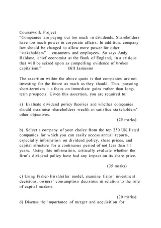
  • 30. 60 $ 717 $ 486 $ 1,746 $ 188,040 $ 352,182 Recall the cost function applying to the high-low and regression methods, which are provided in a variety of forms, depending on the texts you used in your previous math, economics, or accounting courses. Below is a brief outline of the high-low and regression methods. For the high-low method to work, the $H and #H and the $L and #L measures must be from the same accounting period. Preparing Graphs The single cost driver and nonfinancial measure in Table 3 is new retail vehicles sold (NRVS or X in the above cost function). There are eight financial measures (salary; vacation; advertising and training; supplies, tools, and laundry; freight; vehicles; demonstrators; and floor-planning [also known in the automobile retail industry as interest expense relating to new car inventory]), as well as a total (aggregate measure) provided for all eight financial measures (or the Y in the above cost function). Using NRVS, the only available cost-driver, use Excel to prepare nine separate scatter plots and cost function-based trend lines and nine separate line graphs for each of the financial measures provided in Table 3. The images below are an example of completed graphs for salaries. A Scatterplot Graph for Motomart SalariesA Line Graph for Motomart Salaries Now examine, on a preliminary basis, the pattern or trend (or lack thereof) for each of the “X” (NRVS) and “Y” (financial measure) data pairs and consider the following questions: · You’re observing these data pairs for a 60-month period (i.e., five years); are any annual or other seasonal patterns or trends immediately apparent?
  • 31. · Do the slopes of the trend lines (i.e., variable costs) make sense? In the case of salaries (see the graphs above), there’s no apparent trend or pattern. It’s odd that salaries decrease as NRVS increases—in fact, this doesn’t make any sense. However, it’s consistent with the high-low results, which also didn’t make sense. But remember, since this data came from Motomart, the firm attempting to relocate, it’s real and from an actual litigation support engagement (not a textbook problem), so it won’t necessarily work out perfectly. The cost equation in Table 4 shows fixed costs (FC) at $106,866.00 and variable costs to be used to “reduce” total costs (TC) by $110.10 per NRVS. Compare the salary figures and coefficients (in bold type) to the scatterplot graph for Motomart Salaries. Notice that if you extended the trend line in Figure 4, it would hit the y-axis intercept at $106,866.00 (the fixed cost). Also, notice that the R-squared (R-sq) measure in Table 4 equals 4.1 percent. Table 4 SALARY = $106,866.00 – $110.10 NRVS Predictor Coefficient Std Deviation t-statistic p-value Constant 106,866.00 10,793.00 9.90 0.000 NRVS 110.10 70.17 –1.57 0.122 s = 25300 r-sq = 4.1%
  • 32. Analysis of Variance SOURCE DF SS MS F-statistic p-value Regression 1 261,795 261,795 0.10 0.754 Error 58 152,801,120 2,634,502 Total 59 153,062,912 Your math and statistics courses probably reviewed the use of the t-statistic, overall F-statistic, and related p-values, as well as some of the other measures presented here. Our application is a very simple one, so we’ll focus on only the R-squared measure. The other measures are provided in this example only for completeness. Because the high-low technique didn’t work, it makes sense that the regression technique wouldn’t work well, either. Therefore, the results for high-low and regression are consistent. The advantage of the regression technique is that it mathematically quantifies the level of the problem or difficulty with the data. In
  • 33. this case, one of simple regression, the R-squared measure tells the story. Still focusing on the salaries example in Figure 5, the R-squared measure tells us that only 4.1 percent of the total or mixed or semi-fixed cost is explained by NRVS. This means that that cost equation developed from this historical data isn’t helpful in predicting future costs, as nearly 96 percent of the cost behavior, through use of this equation, remains unexplained. Requirements The project requires five steps to be presented. Step 1 – Provide comments on a 5-year Income Statement. Step 2 – Discuss patterns in expense items. Step 3 – Identify High/Low activity levels. Step 4 – Compute cost equations. Step 5 – Summarize your findings. In one Word document, provide individual sections for each Step. This Word document along with the Excel file (described below) will be uploaded when you click on the Take Exam button on your Student Portal to submit your project (described under “Submitting Your Assignment” later in the instructions). This Senior Capstone project highlights your knowledge and the skills you have developed over the course of your education. There is nothing “new” to be learned here. The knowledge and skills required for this project include English Composition, Financial Accounting, Managerial Accounting, Business Statistics and the abilities to think critically and to present your work in a professional manner. If you are unsure or don’t understand something about the project, then go back to your previous subjects to review. For example, if you don’t remember how to use the High/Low Method, the revisit your Managerial Accounting to refresh your memory on how to use the High/Low Method Remember, there is nothing “new” here. Everything about this project you should already know how to do. At the beginning of the assignment, on the right-hand side under "Optional Study Materials" select the "PPMC Excel
  • 34. Spreadsheet" menu item to download the required Excel spreadsheet. · The Excel file provides a detailed example of what needs to be done for one of the expenses in order to fill out the figures required in Steps 3 & 4. You will include this Excel file as part of your project submission along with the Word document you create to present this project. · There is a “60 Months” worksheet that has the 60 months of data already entered. There is also a “Sample” worksheet that an example of how to calculate the R-sq. · There is a “PLOT – SALARY” worksheet that shows how the FC, VC and R-sq figures are calculated for Salary. · There is also a “high&low” worksheet for help with the high/low method in Step 3. · Complete and include the Excel spreadsheet. You will need to create new worksheets for each of the other expenses following the example to calculate the figures needed for Table 5. Operating Profits and Semi-Fixed Expenses Step 1 First, using Tables 2–4, note the pattern of operating profits (or losses) over the five-year period. Then focus only on the semi- fixed expenses contained in Table 2. Do any amounts appear to be odd? (Think about whether the figures are right or wrong. What is it about the individual numbers that is not “right”?) Next, briefly comment on the five-year pattern or trend for operating profit/loss measures. You should be able to respond to this step in a few well-written sentences. Step 2 Focus only on the detailed semi-fixed expense contained in Table 3. Are there any unusual or odd patterns you might note in this detailed financial data? There are 5 expenses that have an oddity about them which doesn’t make sense. Similar to Step 1, what is it about the individual numbers that are not “right”? There are 4 expenses that “stick out” as not being correct and one that has an unusual pattern. attention. You should be able to respond to this requirement in a few well-written sentences.
  • 35. Briefly comment on only the most obvious or apparent measures or patterns, by expense item. Step 3 Identify the high and low measures in each column, just as you would in preparation for the application of the high-low method or technique. For example, in Table 3 the high measure for the cost driver (NRVS) is 280 NRVS in month 13 and the low measure is 31 NRVS in month 12. Repeat this process for each of the eight separate semi-fixed expense columns and also for the total expense column. Insert a table for Step 3 to present your findings. The table should have three columns; 1. Expense 2. High Figure 3. Low Figure After the high and low measures have been identified in each column, try to match each expense column’s high and low measure, separately, to the highs and lows identified in the NRVS column. They won’t match. Don’t try to correct the data, but comment on the potential for application of the high-low technique. What happens when the high and low activity level doesn’t match the high and low expense measure? Does this prevent you from correctly applying the high-low technique? Don’t overanalyze this data, because there’s a problem with it and you don’t have sufficient information to correct it. Merely summarize your observations and unsuccessful attempts to match the high and low NRVS months (identified above), separately, with each of the high and low expense measure months. You should be able to do this in a very few well-written sentences. Step 4 Using the Excel file "Exam 500896 - Motomart Excel Spreadsheet" as per the instructions found above under the "Project Requirements", reproduce and complete the following Table 5 and answer the four questions. The Excel file provides an example of how to arrive at the figures that need to be entered into the Table. You will create new worksheets for each
  • 36. of the remaining expenses. Do the work to arrive at the figures for each expense. Be sure to include the Excel file as part of your submission to "backup" the data presented in the Table in the Word document being submitted. The Excel spreadsheet, while it will be included in your submission for the project, will not be graded. It is supporting documentation for what is being presented in the Word document. Only the information that is in the Word document will be graded. The FC and VC should be rounded to the nearest dollar. The R- sq is a percentage figure carried out to 2 decimal places. Table 5 Column Expense FC VC R-sq 1 Salaries $106,866 –$110 4.10% 2 Vacation 3 Advertising and training 4 Supplies/tools/laundry
  • 37. 5 Freight 6 Vehicles 7 Demonstrators 8 Floor planning Computed total 9 Total Complete the cost equations for the table. Use the R-squared as the single measure of “goodness of fit.” Don’t attempt to improve your results with the elimination of “outliers” or “influential outliers.” As you complete Table 5, answer the following questions:
  • 38. 1. What problems did you encounter? 2. Are the R-squared measures high or low? 3. Are the slopes negative or positive? 4. Are your conclusions consistent with those from the high-low effort? Step 5 Summarize your findings by answering the following questions: 1. Can the Motomart data be used to prepare a reliable financial forecast? Why or why not? 2. If Motomart is included in the very large database used to prepare the financial forecast that supports the relocation of Motomart closer to Existing Dealer, what concerns might present themselves with respect to the remainder of the database used for this forecast? 3. Would you rely on this forecast? Writing Guidelines Refer to the “Submitting Your Work” section at the end of this book for details on submission requirements for the Motomart Case assignment. Grading Criteria Your assignment will be evaluated according to the following criteria: Content 80 percent Written Communication 10 percent Format 10 percent Criteria Grade Content 80 pts · Step 1 – Provides comments on 5-year income statement (worth 10 points) · Step 2 – Discuss patterns in expense items (worth 10 points) · Step 3 – Identify high and low activity levels (worth 10
  • 39. points) · Step 4 – Compute cost equations (worth 30 points) · Step 5 – Summarize your findings (worth 20 points) Written Communication 10 pts · Answers each question in complete sentences leading to well - structured responses to each Step listed above. · Uses correct grammar, spelling, punctuation, and sentence structure · Provides clear organization by using words like first, however, on the other hand, and so on, consequently, since, next, and when · Makes sure the paper contains no typographical errors Format 10 pts The paper is double-spaced, typed in font size 12. It includes the student’s · Name and address · Student number, Course title and number, and project number Total Grade % Submitting Your Work Writing Guidelines 1. Type your submission, double-spaced, in a standard print font, size 12. Use a standard document format with 1-inch margins. (Do not use any fancy or cursive fonts.) 2. Include the following information at the top of your paper: a. Name and complete mailing address b. Student number c. Course title and number (Senior Capstone: Business, BUS 450) d. Project number (see Format instructions) e. Project title (Professional Development Activity, Case 1, etc.) 3. Read the assignments carefully and complete each one in the order given.
  • 40. 4. Be specific. Limit your submission to the questions asked and issues mentioned. 5. If you include quotes or ideas from textbooks or other sources, provide a reference page in either APA or MLA style. On this page, list books, Web sites, journals, or any other references used in preparing the paper. 6. Proofread your work carefully. Check for correct spelling, grammar, punctuation, and capitalization. NOTES Top of Form Bottom of Form READING ASSIGNMENT Your project must be submitted as a Word document (.docx, .doc)*. Your project will be individually graded by your instructor and therefore will take up to a few weeks to grade. Be sure that each of your files contains the following information: · Your name · Your student ID number · The exam number · Your email address To submit your graded project, follow these steps: · Log in to your student portal. · Click on Take Exam next to the lesson you’re working on. · Find the exam number for your project at the top of the Project Upload page. · Follow the instructions provided to complete your exam. Be sure to keep a backup copy of any files you submit to the school!
  • 41. This case is based on real financial data provided by a retail automobile dealership (Motomart) seeking to relocate closer to an existing retail dealership. You’ll examine the mixed cost data from Motomart and apply both high-low and regression to attempt to separate mixed costs into their fixed and variable components for break-even and contribution margin computations. You’ll find that the data is flawed because Motomart was a single observation in a larger database. Don’t attempt to correct the data (e.g., remove outliers or influential outliers). You’ll be producing a scatterplot and apply high-low and regression methods to the extent practicable and writing a summary report of the findings. Motomart operates a retail automobile dealership. The manufacturer of Motomart products, like all automobile manufacturers, produces forecasts. It has long been an industry practice to use variable costing-based/break-even analyses as the foundation for these forecasts, to examine their cost behavior as it relates to the new retail vehicles sold (NRVS) cost driver. In preparing this financial information, a common financial statement format and accounting procedures manual are provided to each retail auto dealership. The dealership is required to produce monthly financial statements using the guidelines provided by this common accounting procedures manual, and then furnish these financial statements to the manufacturer. General Motors, Ford, Nissan, and all other automobile manufacturers employ similar procedures manuals. The use of a common format facilitates the development of composite financial statements that can be used to estimate costs and produce financial forecasts for future or proposed retail dealership sites (Cataldo and Kruck 1998). Zimmerman (2003) suggests that as many as 77 percents of manufacturers divide costs into variable and fixed components and that managers arrive at these estimates by classifying individual accounts as being primarily fixed or primarily variable (67). For this case, you’ll examine mixed costs as defined by the manufacturer. Using the scatterplot, high-low, and regression
  • 42. methods, separate these mixed costs into their fixed and variable components. The data is problematic, and a clear solution won’t exist. Don’t attempt to correct the data by removing outliers, but make observations based on any patterns you observe. The case will expose you to actual data and require you to summarize your findings, including any conclusions you’re able to reach and why the financial data makes it impossible to separate the mixed costs into their fixed and variable components. Motomart: A Litigation Support Engagement The Motomart case evolved from a litigation support engagement. The lead author of this case was hired to analyze the data and provide expert testimony. His report and testimony was made available to the public (for a fee to cover reproduction costs). A broad description of the relevant points for the Motomart case follows. Motomart wanted to move their retail automobile dealership, blaming their location for declining profits and increasing losses. They provided financial projections, using variable costing, to show that after the relocation both Motomart and the existing dealership would be profitable. They created these financial projections using a database provided by the manufacturer, which included all North American retail automobile dealerships. Motomart was one of the observations or retail automobile dealerships included in the database used to create these financial projections. You’ll be examining portions of Motomart’s historical financial data. The relocation site was quite close to the existing dealership (which we’ll refer to as Existing Dealer), and Existing Dealer felt that, if the relocation was permitted, one or both of the dealerships would fail to break even and eventually go bankrupt, leading to poor service, or what the industry refers to as “orphaned” owners of these automobiles. Antitrust laws provided Existing Dealer with the means to block the relocation requested by Motomart, but only if it could prove that the relocation wasn’t in the best interest of the consuming
  • 43. public. Generally, the only way to prove this is to prove that there’s simply not enough business for both retail automobile dealerships to break even (or generate a reasonable return on investment, given the risks associated with the industry). Again, the manufacturer, in support of the proposed Motomart relocation, supplied financial projections showing that both retail automobile dealerships would be profitable after the relocation. The expert witness hired to investigate the merits of the relocation was given the Motomart data, but not the entire database that included the Motomart data. The Motomart data was in such poor form that it wasn’t possible to produce a financial forecast. An alternative forecast, not included in this case, was produced. This alternative forecast did not support the relocation of Motomart to a site closer to Existing Dealer. The alternative forecast showed that the market simply couldn’t support two retail automobile dealerships. The implication was that, as the weaker of the two dealerships, Motomart was losing business to Existing Dealer. In conclusion, the relocation request by Motomart was denied. Income and Expense Data The following tables give you information such as income statements, semi-fixed expenses, and salaries for Motomart. Look for unusual entries or discrepancies in their records and, where you can, note the cause of the problems. Table 3 summarizes financial and cost driver information produced by Motomart, where new retail vehicles sold (NRVS) is the cost driver. The account classification method has resulted in three cost behavior classifications: variable, semi- fixed, and fixed costs. Semi-fixed is the automobile industry- specific term used for mixed costs. We’ll assume that Motomart’s classifications of variable costs (VCs) and fixed costs (FCs) are correct, and focus our analysis on Motomart’s semi-fixed or mixed costs. Table 2 SElECTED HISTORICAl INCOME STATEMENT AND
  • 44. RElATED MEASURES 1984 1985 1986 1987 1988 Net Variable Revenues* 2,885,969 3,828,255 4,086,667 3,940,799 4,298,748 Semi-Fixed (S-F) Expenses: Salaries 613,006 968,789 1,211,464 1,289,758 1,360,489 Vacation 600 26,705 19,468 19,059 18,268 Advertising & Training 210,226 288,347 281,219 309,608 371,314 Supplies/Tools/Laundry 31,473 46,141 75,468
  • 46. 2,290,867 2,164,362 2,653,620 Operating Profit/(Loss)** 263,828 112,314 -96,699 -94,345 -516,092 New Retail Vehicles Sold 1,798 1,977 1,674 1,450 1,897 Notes: * Revenues less variable costs equal Net Variable Revenues (or Contribution Margin, in aggregate). ** Net Variable Revenue less Total S-F Expenses less Total Fixed Expenses equals Operating Profit/(Loss). Table 3 provides five years of monthly data (N=60) for NRVS and the related semi-fixed or mixed cost measures. Semifixed costs were significant. Recall that they ranged from nearly $1.2 million for calendar and fiscal year (FY) 1984 to almost $2.2 million for FY 1988 (see Table 2). Table 3 SEMI-FIXED (MIXED) EXPENSES FOR THE 60-MONTH PERIOD (FY 1984 THROUGH 1988) Mo NRVS Salary Vacation Adv/Trng SplyTls/Lndry 1 197
  • 47. $ 52,951 $ - $ 22,561 $ 1,118 2 133 $ 47,054 $ - $ 19,040 $ 3,573 3 132 $ 55,372 $ - $ 14,373 $ 1,388 4 141 $ 46,114 $ - $ 15,022 $ 2,894 5 182 $ 48,309 $ - $ 19,966 $ 1,896 6 156 $ 49,643 $ - $ 12,019 $ 1,188 7 196
  • 48. $ 55,784 $ 300 $ 13,217 $ 3,912 8 178 $ 47,957 $ - $ 17,303 $ 2,012 9 159 $ 53,743 $ - $ 16,535 $ 2,717 10 141 $ 53,109 $ - $ 23,821 $ 1,102 11 152 $ 45,491 $ 300 $ 14,146 $ 2,630 12 31 $ 57,479 $ - $ 22,223 $ 7,043 13 280
  • 49. $ 49,049 $ - $ 19,992 $ 1,999 14 136 $ 46,698 $ 300 $ 20,251 $ 1,192 15 174 $ 59,790 $ 200 $ 20,082 $ 1,336 16 171 $ 80,773 $ 600 $ 26,716 $ 3,873 17 167 $ 71,130 $ 9,212 $ 25,223 $ 5,560 18 161 $ 82,490 $ 6,007 $ 21,106 $ 1,737 19 173
  • 50. $ 98,172 $ 500 $ 17,799 $ 1,847 20 161 $ 90,685 $ 2,690 $ 28,038 $ 4,415 21 167 $ 97,771 $ 600 $ 37,284 $ 2,827 22 153 $ 87,129 $ 1,740 $ 24,236 $ 5,836 23 201 $ 95,910 $ 2,074 $ 27,244 $ 3,387 24 33 $ 09,192 $ 2,782 $ 20,376 $ 12,132 25 227
  • 51. $ 89,041 $ 1,880 $ 26,719 $ 4,383 26 150 $ 92,165 $ 3,602 $ 14,727 $ 10,231 27 142 $ 88,981 $ 744 $ 27,880 $ 7,734 28 104 $ 95,898 $ 960 $ 21,872 $ (684) 29 121 $ 96,245 $ - $ 18,705 $ 8,329 30 99 $ 106,364 $ - $ 23,835 $ 2,540 31 150
  • 52. $ 90,564 $ 1,950 $ 25,605 $ 5,862 32 144 $ 98,418 $ 1,540 $ 17,763 $ 6,998 33 154 $ 110,436 $ 2,693 32,379 $ 8,131 34 130 $ 102,042 $ 1,060 $ 19,324 $ 6,026 35 202 $ 124,413 $ 3,519 $ 22,412 $ 9,120 36 51 $ 116,897 $ 1,520 $ 29,998 $ 6,798 37 148
  • 53. $ 97,083 $ 1,080 $ 9,112 $ 6,627 38 153 $ 104,727 $ 3,230 $ 38,616 $ 5,892 39 83 $ 95,622 $ 953 $ 22,690 $ 3,450 40 101 $ 96,438 $ 1,244 $ 14,703 $ 5,259 41 140 $ 114,995 $ - $ 28,764 $ 2,294 42 132 $ 105,337 $ 160 $ 27,253 $ 8,155 43 112
  • 54. $ 98,989 $ 2,480 $ 24,419 $ 1,621 44 127 $ 124,352 $ 1,800 $ 26,011 $ 902 45 139 $ 115,875 $ 1,417 $ 24,492 $ 5,158 46 156 $ 113,035 $ 1,820 $ 31,158 $ 2,901 47 126 $ 119,106 $ 3,338 $ 32,213 $ 14,426 48 33 $ 104,199 $ 1,537 $ 30,177 $ 9,250 49 209
  • 55. $ 98,938 $ 1,866 $ 26,737 $ 1,694 50 124 $ 108,606 $ 3,676 $ 31,084 $ 9,040 51 131 $ 106,396 $ 1,197 $ 33,278 $ 2,099 52 144 $ 106,778 $ 241 $ 32,657 $ 9,328 53 93 $ 124,805 $ 500 $ 29,794 $ 4,268 54 199 $ 110,153 $ 1,910 $ 38,431 $ 5,407 55 170
  • 56. $ 117,276 $ 800 $ 27,640 $ 9,305 56 186 $ 112,055 $ 980 $ 28,657 $ 1,803 57 200 $ 114,765 $ 1,695 $ 36,425 $ 8,839 58 146 $ 128,007 $ 1,560 $ 27,720 $ 10,944 59 222 $ 116,811 $ 2,249 $ 27,941 $ 5,775 60 73 $ 115,899 $ 1,594 $ 30,950 $ 30,950 Table 3 Continued
  • 57. SEMI-FIXED (MIXED) EXPENSES FOR THE 60-MONTH PERIOD (FY 1984 THROUGH 1988) Mo Freight Vehicles Demo's Floor-Plan Total 1 $ 382 $ 2,052 $ 1,881 $ (78,173) $ 2,772 2 $ 409 $ 1,405 $ 695 $ 28,456 $ 100,632 3 $ 742 $ 1,380 $ 469 $ 34,423 $ 108,147 4 $ 675 $ 2,057 $ 125 $ 5,697 $ 72,584 5 $ 572 $ 1,603 $ 131
  • 58. $ 34,599 $ 107,076 6 $ 407 $ 2,524 $ 1,229 $ 53,737 $ 120,747 7 $ 643 $ 2,348 $ 1,206 $ 5,507 $ 82,917 8 $ 605 $ 1,208 $ 436 $ 32,436 $ 101,957 9 $ 209 $ 2,400 $ 1,476 $ 28,950 $ 106,030 10 $ 184 $ 2,076 $ 1,168 $ 20,876 $ 102,336 11 $ 331 $ 1,677 $ 635
  • 59. $ 45,278 $ 110,488 12 $ 560 $ 2,183 $ 1,014 $ 66,745 $ 157,247 13 $ 582 $ 1,927 $ (477) $ (30,104) $ 42,968 14 $ 603 $ 1,156 $ 1,839 $ 50,583 $ 122,622 15 $ 492 $ 1,898 $ 1,260 $ 18,803 $ 103,861 16 $ 559 $ 1,808 $ 510 $ 23,080 $ 137,919 17 $ 356 $ 1,816 $ 2,350
  • 60. $ 18,774 $ 134,421 18 $ 439 $ 1,384 $ (288) $ 23,802 $ 136,677 19 $ 1,628 $ 1,962 $ 1,591 $ 33,848 $ 157,347 20 $ (12) $ 2,446 $ (3,308) $ 13,480 $ 138,434 21 $ 480 $ 2,296 $ 1,709 $ 22,965 $ 165,932 22 $ 79 $ 3,175 $ 798 $ 18,898 $ 141,891 23 $ 188 $ 1,287 $ (2,025)
  • 61. $ 38,699 $ 166,764 24 $ 593 $ 2,563 $ 1,010 $ 68,285 $ 216,933 25 $ 769 $ 2,205 $ 2,493 $ (44,140) $ 83,350 26 $ 593 $ 2,289 $ (2,051) $ 36,311 $ 157,867 27 $ 414 $ 1,891 $ 386 $ 19,865 $ 147,895 28 $ 425 $ 2,288 $ 178 $ 19,013 $ 139,950 29 $ 483 $ 2,223 $ (262)
  • 62. $ 16,228 $ 141,951 30 $ 417 $ 1,683 $ (1,356) $ 37,637 $ 171,120 31 $ 222 $ 1,586 $ 486 $ (1,121) $ 125,154 32 $ 49 $ 1,751 $ (1,924) $ 34,757 $ 159,352 33 $ 818 $ 2,082 $ 1,547 $ 26,419 $ 184,505 34 $ 1,015 $ 1,714 $ 132 $ 21,134 $ 52,447 35 $ 1,255 $ 2,173 $ (2,337)
  • 63. $ 18,578 $ 179,133 36 $ 68 $ 1,779 $ 1,195 $ 91,520 $ 249,775 37 $ 565 $ 1,324 $ 1,164 $ (73,753) $ 43,202 38 $ 369 $ 1,523 $ (1,839) $ 30,443 $ 182,961 39 $ (182) $ 2,087 $ 454 $ 17,725 $ 142,799 40 $ 709 $ 2,095 $ 868 $ 26,402 $ 147,718 41 $ 1,006 $ 1,304 $ (1,990)
  • 64. $ (3,789 $ 142,584 42 $ 521 $ 1,667 $ 1,869 $ 15,090 $ 160,052 43 $ 514 $ 1,040 $ 329 $ (945) $ 128,447 44 $ 917 $ 2,880 $ (1,897) $ 30,405 $ 185,370 45 $ (77 $ 1,281 $ 2,959 $ 14,781 $ 165,886 46 $ 450 $ 2,259 $ 417 $ 15,613 $ 167,653 47 $ 120 $ 1,394 $ (2,659)
  • 65. $ 40,968 $ 208,906 48 $ 819 $ 1,516 $ 4,517 $ 43,189 $ 195,204 49 $ 853 $ 1,657 $ 601 $ (20,127) $ 112,219 50 $ 498 $ 2,266 $ (284) $ 18,236 $ 173,122 51 $ 605 $ 1,952 $ 668 $ 15,176 $ 161,371 52 $ 483 $ 1,852 $ 1,409 $ 25,245 $ 177,993 53 $ 788 $ 1,704 $ (1,771)
  • 66. $ 6,493 $ 166,581 54 $ 529 $ 1,882 $ 453 $ 21,851 $ 180,616 55 $ (180) $ 977 $ 1,310 $ 7 $ 157,135 56 $ 242) $ 846 $ (2,844) $ 17,192 $ 158,447 57 $ 859 $ 2,856 $ 1,532 $ 14,864 $ 181,835 58 $ (492) $ 1,864 $ 1,400 $ 10,121 $ 181,124 59 $ 245 $ 1,141 $ (3,513)
  • 67. $ 7,946 $ 158,595 60 $ 717 $ 486 $ 1,746 $ 188,040 $ 352,182 Recall the cost function applying to the high-low and regression methods, which are provided in a variety of forms, depending on the texts you used in your previous math, economics, or accounting courses. Below is a brief outline of the high-low and regression methods. For the high-low method to work, the $H and #H and the $L and #L measures must be from the same accounting period. Preparing Graphs The single cost driver and nonfinancial measure in Table 3 is new retail vehicles sold (NRVS or X in the above cost function). There are eight financial measures (salary; vacation; advertising and training; supplies, tools, and laundry; freight; vehicles; demonstrators; and floor-planning [also known in the automobile retail industry as interest expense relating to new car inventory]), as well as a total (aggregate measure) provided for all eight financial measures (or the Y in the above cost function). Using NRVS, the only available cost-driver, use Excel to prepare nine separate scatter plots and cost function-based trend lines and nine separate line graphs for each of the financial measures provided in Table 3. The images below are an example of completed graphs for salaries. A Scatterplot Graph for Motomart SalariesA Line Graph for Motomart Salaries Now examine, on a preliminary basis, the pattern or trend (or lack thereof) for each of the “X” (NRVS) and “Y” (financial measure) data pairs and consider the following questions: · You’re observing these data pairs for a 60-month period (i.e.,
  • 68. five years); are any annual or other seasonal patterns or trends immediately apparent? · Do the slopes of the trend lines (i.e., variable costs) make sense? In the case of salaries (see the graphs above), there’s no apparent trend or pattern. It’s odd that salaries decrease as NRVS increases—in fact, this doesn’t make any sense. However, it’s consistent with the high-low results, which also didn’t make sense. But remember, since this data came from Motomart, the firm attempting to relocate, it’s real and from an actual litigation support engagement (not a textbook problem), so it won’t necessarily work out perfectly. The cost equation in Table 4 shows fixed costs (FC) at $106,866.00 and variable costs to be used to “reduce” total costs (TC) by $110.10 per NRVS. Compare the salary figures and coefficients (in bold type) to the scatterplot graph for Motomart Salaries. Notice that if you extended the trend line in Figure 4, it would hit the y-axis intercept at $106,866.00 (the fixed cost). Also, notice that the R-squared (R-sq) measure in Table 4 equals 4.1 percent. Table 4 SALARY = $106,866.00 – $110.10 NRVS Predictor Coefficient Std Deviation t-statistic p-value Constant 106,866.00 10,793.00 9.90 0.000 NRVS 110.10 70.17 –1.57
  • 69. 0.122 s = 25300 r-sq = 4.1% Analysis of Variance SOURCE DF SS MS F-statistic p-value Regression 1 261,795 261,795 0.10 0.754 Error 58 152,801,120 2,634,502 Total 59 153,062,912 Your math and statistics courses probably reviewed the use of the t-statistic, overall F-statistic, and related p-values, as well as some of the other measures presented here. Our application is a very simple one, so we’ll focus on only the R-squared measure. The other measures are provided in this example only for completeness. Because the high-low technique didn’t work, it makes sense that the regression technique wouldn’t work well, either. Therefore, the results for high-low and regression are consistent. The
  • 70. advantage of the regression technique is that it mathematically quantifies the level of the problem or difficulty with the data. In this case, one of simple regression, the R-squared measure tells the story. Still focusing on the salaries example in Figure 5, the R-squared measure tells us that only 4.1 percent of the total or mixed or semi-fixed cost is explained by NRVS. This means that that cost equation developed from this historical data isn’t helpful in predicting future costs, as nearly 96 percent of the cost behavior, through use of this equation, remains unexplained. Requirements The project requires five steps to be presented. Step 1 – Provide comments on a 5-year Income Statement. Step 2 – Discuss patterns in expense items. Step 3 – Identify High/Low activity levels. Step 4 – Compute cost equations. Step 5 – Summarize your findings. In one Word document, provide individual sections for each Step. This Word document along with the Excel file (described below) will be uploaded when you click on the Take Exam button on your Student Portal to submit your project (described under “Submitting Your Assignment” later in the instructions). This Senior Capstone project highlights your knowledge and the skills you have developed over the course of your education. There is nothing “new” to be learned here. The knowledge and skills required for this project include English Composition, Financial Accounting, Managerial Accounting, Business Statistics and the abilities to think critically and to present your work in a professional manner. If you are unsure or don’t understand something about the project, then go back to your previous subjects to revi ew. For example, if you don’t remember how to use the High/Low Method, the revisit your Managerial Accounting to refresh your memory on how to use the High/Low Method Remember, there is nothing “new” here. Everything about this project you should already know how to do.
  • 71. At the beginning of the assignment, on the right-hand side under "Optional Study Materials" select the "PPMC Excel Spreadsheet" menu item to download the required Excel spreadsheet. · The Excel file provides a detailed example of what needs to be done for one of the expenses in order to fill out the figures required in Steps 3 & 4. You will include this Excel file as part of your project submission along with the Word document you create to present this project. · There is a “60 Months” worksheet that has the 60 months of data already entered. There is also a “Sample” worksheet that an example of how to calculate the R-sq. · There is a “PLOT – SALARY” worksheet that shows how the FC, VC and R-sq figures are calculated for Salary. · There is also a “high&low” worksheet for help with the high/low method in Step 3. · Complete and include the Excel spreadsheet. You will need to create new worksheets for each of the other expenses following the example to calculate the figures needed for Table 5. Operating Profits and Semi-Fixed Expenses Step 1 First, using Tables 2–4, note the pattern of operating profits (or losses) over the five-year period. Then focus only on the semi- fixed expenses contained in Table 2. Do any amounts appear to be odd? (Think about whether the figures are right or wrong. What is it about the individual numbers that is not “right”?) Next, briefly comment on the five-year pattern or trend for operating profit/loss measures. You should be able to respond to this step in a few well-written sentences. Step 2 Focus only on the detailed semi-fixed expense contained in Table 3. Are there any unusual or odd patterns you might note in this detailed financial data? There are 5 expenses that have an oddity about them which doesn’t make sense. Similar to Step 1, what is it about the individual numbers that are not “right”? There are 4 expenses that “stick out” as not being correct and
  • 72. one that has an unusual pattern. attention. You should be able to respond to this requirement in a few well-written sentences. Briefly comment on only the most obvious or apparent measures or patterns, by expense item. Step 3 Identify the high and low measures in each column, just as you would in preparation for the application of the high-low method or technique. For example, in Table 3 the high measure for the cost driver (NRVS) is 280 NRVS in month 13 and the low measure is 31 NRVS in month 12. Repeat this process for each of the eight separate semi-fixed expense columns and also for the total expense column. Insert a table for Step 3 to present your findings. The table should have three columns; 1. Expense 2. High Figure 3. Low Figure After the high and low measures have been identified in each column, try to match each expense column’s high and low measure, separately, to the highs and lows identified in the NRVS column. They won’t match. Don’t try to correct the data, but comment on the potential for application of the high-low technique. What happens when the high and low activity level doesn’t match the high and low expense measure? Does this prevent you from correctly applying the high-low technique? Don’t overanalyze this data, because there’s a problem with it and you don’t have sufficient information to correct it. Merely summarize your observations and unsuccessful attempts to match the high and low NRVS months (identified above), separately, with each of the high and low expense measure months. You should be able to do this in a very few well-written sentences. Step 4 Using the Excel file "Exam 500896 - Motomart Excel Spreadsheet" as per the instructions found above under the "Project Requirements", reproduce and complete the following Table 5 and answer the four questions. The Excel file provides
  • 73. an example of how to arrive at the figures that need to be entered into the Table. You will create new worksheets for each of the remaining expenses. Do the work to arrive at the figures for each expense. Be sure to include the Excel file as part of your submission to "backup" the data presented in the Table in the Word document being submitted. The Excel spreadsheet, while it will be included in your submission for the project, will not be graded. It is supporting documentation for what is being presented in the Word document. Only the information that is in the Word document will be graded. The FC and VC should be rounded to the nearest dollar. The R- sq is a percentage figure carried out to 2 decimal places. Table 5 Column Expense FC VC R-sq 1 Salaries $106,866 –$110 4.10% 2 Vacation 3 Advertising and training 4 Supplies/tools/laundry
  • 74. 5 Freight 6 Vehicles 7 Demonstrators 8 Floor planning Computed total 9 Total Complete the cost equations for the table. Use the R-squared as the single measure of “goodness of fit.” Don’t attempt to improve your results with the elimination of “outliers” or
  • 75. “influential outliers.” As you complete Table 5, answer the following questions: 1. What problems did you encounter? 2. Are the R-squared measures high or low? 3. Are the slopes negative or positive? 4. Are your conclusions consistent with those from the high-low effort? Step 5 Summarize your findings by answering the following questions: 1. Can the Motomart data be used to prepare a reliable financial forecast? Why or why not? 2. If Motomart is included in the very large database used to prepare the financial forecast that supports the relocation of Motomart closer to Existing Dealer, what concerns might present themselves with respect to the remainder of the database used for this forecast? 3. Would you rely on this forecast? Writing Guidelines Refer to the “Submitting Your Work” section at the end of this book for details on submission requirements for the Motomart Case assignment. Grading Criteria Your assignment will be evaluated according to the followi ng criteria: Content 80 percent Written Communication 10 percent Format 10 percent Criteria Grade Content 80 pts · Step 1 – Provides comments on 5-year income statement (worth 10 points)
  • 76. · Step 2 – Discuss patterns in expense items (worth 10 points) · Step 3 – Identify high and low activity levels (worth 10 points) · Step 4 – Compute cost equations (worth 30 points) · Step 5 – Summarize your findings (worth 20 points) Written Communication 10 pts · Answers each question in complete sentences leading to well- structured responses to each Step listed above. · Uses correct grammar, spelling, punctuation, and sentence structure · Provides clear organization by using words like first, however, on the other hand, and so on, consequently, since, next, and when · Makes sure the paper contains no typographical errors Format 10 pts The paper is double-spaced, typed in font size 12. It includes the student’s · Name and address · Student number, Course title and number, and project number Total Grade % Submitting Your Work Writing Guidelines 1. Type your submission, double-spaced, in a standard print font, size 12. Use a standard document format with 1-inch margins. (Do not use any fancy or cursive fonts.) 2. Include the following information at the top of your paper: a. Name and complete mailing address b. Student number c. Course title and number (Senior Capstone: Business, BUS 450) d. Project number (see Format instructions) e. Project title (Professional Development Activity, Case 1, etc.)
  • 77. 3. Read the assignments carefully and complete each one in the order given. 4. Be specific. Limit your submission to the questions asked and issues mentioned. 5. If you include quotes or ideas from textbooks or other sources, provide a reference page in either APA or MLA style. On this page, list books, Web sites, journals, or any other references used in preparing the paper. 6. Proofread your work carefully. Check for correct spelling, grammar, punctuation, and capitalization. NOTES Top of Form Bottom of Form READING ASSIGNMENT Your project must be submitted as a Word document (.docx, .doc)*. Your project will be individually graded by your instructor and therefore will take up to a few weeks to grade. Be sure that each of your files contains the following information: · Your name · Your student ID number · The exam number · Your email address To submit your graded project, follow these steps: · Log in to your student portal. · Click on Take Exam next to the lesson you’re working on. · Find the exam number for your project at the top of the Project Upload page. · Follow the instructions provided to complete your exam.
  • 78. Be sure to keep a backup copy of any files you submit to the school! This case is based on real financial data provided by a retail automobile dealership (Motomart) seeking to relocate closer to an existing retail dealership. You’ll examine the mixed cost data from Motomart and apply both high-low and regression to attempt to separate mixed costs into their fixed and variable components for break-even and contribution margin computations. You’ll find that the data is flawed because Motomart was a single observation in a larger database. Don’t attempt to correct the data (e.g., remove outliers or influential outliers). You’ll be producing a scatterplot and apply hi gh-low and regression methods to the extent practicable and writing a summary report of the findings. Motomart operates a retail automobile dealership. The manufacturer of Motomart products, like all automobile manufacturers, produces forecasts. It has long been an industry practice to use variable costing-based/break-even analyses as the foundation for these forecasts, to examine their cost behavior as it relates to the new retail vehicles sold (NRVS) cost driver. In preparing this financial information, a common financial statement format and accounting procedures manual are provided to each retail auto dealership. The dealership is required to produce monthly financial statements using the guidelines provided by this common accounting procedures manual, and then furnish these financial statements to the manufacturer. General Motors, Ford, Nissan, and all other automobile manufacturers employ similar procedures manuals. The use of a common format facilitates the development of composite financial statements that can be used to estimate costs and produce financial forecasts for future or proposed retail dealership sites (Cataldo and Kruck 1998). Zimmerman (2003) suggests that as many as 77 percents of manufacturers divide costs into variable and fixed compone nts and that managers arrive at these estimates by classifying individual accounts as being primarily fixed or primarily variable (67).
  • 79. For this case, you’ll examine mixed costs as defined by the manufacturer. Using the scatterplot, high-low, and regression methods, separate these mixed costs into their fixed and variable components. The data is problematic, and a clear solution won’t exist. Don’t attempt to correct the data by removing outliers, but make observations based on any patterns you observe. The case will expose you to actual data and require you to summarize your findings, including any conclusions you’re able to reach and why the financial data makes it impossible to separate the mixed costs into their fixed and variable components. Motomart: A Litigation Support Engagement The Motomart case evolved from a litigation support engagement. The lead author of this case was hired to analyze the data and provide expert testimony. His report and testimony was made available to the public (for a fee to cover reproduction costs). A broad description of the relevant points for the Motomart case follows. Motomart wanted to move their retail automobile dealership, blaming their location for declining profits and increasing losses. They provided financial projections, using variable costing, to show that after the relocation both Motomart and the existing dealership would be profitable. They created these financial projections using a database provided by the manufacturer, which included all North American retail automobile dealerships. Motomart was one of the observations or retail automobile dealerships included in the database used to create these financial projections. You’ll be examining portions of Motomart’s historical financial data. The relocation site was quite close to the existing dealership (which we’ll refer to as Existing Dealer), and Existing Dealer felt that, if the relocation was permitted, one or both of the dealerships would fail to break even and eventually go bankrupt, leading to poor service, or what the industry refers to as “orphaned” owners of these automobiles. Antitrust laws provided Existing Dealer with the means to block
  • 80. the relocation requested by Motomart, but only if it could prove that the relocation wasn’t in the best interest of the consuming public. Generally, the only way to prove this is to prove that there’s simply not enough business for both retail automobile dealerships to break even (or generate a reasonable return on investment, given the risks associated with the industry). Again, the manufacturer, in support of the proposed Motomart relocation, supplied financial projections showing that both retail automobile dealerships would be profitable after the relocation. The expert witness hired to investigate the merits of the relocation was given the Motomart data, but not the entire database that included the Motomart data. The Motomart data was in such poor form that it wasn’t possible to produce a financial forecast. An alternative forecast, not included in this case, was produced. This alternative forecast did not support the relocation of Motomart to a site closer to Existing Dealer. The alternative forecast showed that the market simply couldn’t support two retail automobile dealerships. The implication was that, as the weaker of the two dealerships, Motomart was losing business to Existing Dealer. In conclusion, the relocation request by Motomart was denied. Income and Expense Data The following tables give you information such as income statements, semi-fixed expenses, and salaries for Motomart. Look for unusual entries or discrepancies in their records and, where you can, note the cause of the problems. Table 3 summarizes financial and cost driver information produced by Motomart, where new retail vehicles sold (NRVS) is the cost driver. The account classification method has resulted in three cost behavior classifications: variable, semi - fixed, and fixed costs. Semi-fixed is the automobile industry- specific term used for mixed costs. We’ll assume that Motomart’s classifications of variable costs (VCs) and fixed costs (FCs) are correct, and focus our analysis on Motomart’s semi-fixed or mixed costs.
  • 81. Table 2 SElECTED HISTORICAl INCOME STATEMENT AND RElATED MEASURES 1984 1985 1986 1987 1988 Net Variable Revenues* 2,885,969 3,828,255 4,086,667 3,940,799 4,298,748 Semi-Fixed (S-F) Expenses: Salaries 613,006 968,789 1,211,464 1,289,758 1,360,489 Vacation 600 26,705 19,468 19,059 18,268 Advertising & Training 210,226 288,347 281,219 309,608 371,314 Supplies/Tools/Laundry 31,473
  • 83. 1,449,208 2,050,172 2,290,867 2,164,362 2,653,620 Operating Profit/(Loss)** 263,828 112,314 -96,699 -94,345 -516,092 New Retail Vehicles Sold 1,798 1,977 1,674 1,450 1,897 Notes: * Revenues less variable costs equal Net Variable Revenues (or Contribution Margin, in aggregate). ** Net Variable Revenue less Total S-F Expenses less Total Fixed Expenses equals Operating Profit/(Loss). Table 3 provides five years of monthly data (N=60) for NRVS and the related semi-fixed or mixed cost measures. Semifixed costs were significant. Recall that they ranged from nearly $1.2 million for calendar and fiscal year (FY) 1984 to almost $2.2 million for FY 1988 (see Table 2). Table 3 SEMI-FIXED (MIXED) EXPENSES FOR THE 60-MONTH PERIOD (FY 1984 THROUGH 1988) Mo NRVS Salary Vacation Adv/Trng SplyTls/Lndry
  • 84. 1 197 $ 52,951 $ - $ 22,561 $ 1,118 2 133 $ 47,054 $ - $ 19,040 $ 3,573 3 132 $ 55,372 $ - $ 14,373 $ 1,388 4 141 $ 46,114 $ - $ 15,022 $ 2,894 5 182 $ 48,309 $ - $ 19,966 $ 1,896 6 156 $ 49,643 $ - $ 12,019 $ 1,188
  • 85. 7 196 $ 55,784 $ 300 $ 13,217 $ 3,912 8 178 $ 47,957 $ - $ 17,303 $ 2,012 9 159 $ 53,743 $ - $ 16,535 $ 2,717 10 141 $ 53,109 $ - $ 23,821 $ 1,102 11 152 $ 45,491 $ 300 $ 14,146 $ 2,630 12 31 $ 57,479 $ - $ 22,223 $ 7,043
  • 86. 13 280 $ 49,049 $ - $ 19,992 $ 1,999 14 136 $ 46,698 $ 300 $ 20,251 $ 1,192 15 174 $ 59,790 $ 200 $ 20,082 $ 1,336 16 171 $ 80,773 $ 600 $ 26,716 $ 3,873 17 167 $ 71,130 $ 9,212 $ 25,223 $ 5,560 18 161 $ 82,490 $ 6,007 $ 21,106 $ 1,737
  • 87. 19 173 $ 98,172 $ 500 $ 17,799 $ 1,847 20 161 $ 90,685 $ 2,690 $ 28,038 $ 4,415 21 167 $ 97,771 $ 600 $ 37,284 $ 2,827 22 153 $ 87,129 $ 1,740 $ 24,236 $ 5,836 23 201 $ 95,910 $ 2,074 $ 27,244 $ 3,387 24 33 $ 09,192 $ 2,782 $ 20,376 $ 12,132
  • 88. 25 227 $ 89,041 $ 1,880 $ 26,719 $ 4,383 26 150 $ 92,165 $ 3,602 $ 14,727 $ 10,231 27 142 $ 88,981 $ 744 $ 27,880 $ 7,734 28 104 $ 95,898 $ 960 $ 21,872 $ (684) 29 121 $ 96,245 $ - $ 18,705 $ 8,329 30 99 $ 106,364 $ - $ 23,835 $ 2,540
  • 89. 31 150 $ 90,564 $ 1,950 $ 25,605 $ 5,862 32 144 $ 98,418 $ 1,540 $ 17,763 $ 6,998 33 154 $ 110,436 $ 2,693 32,379 $ 8,131 34 130 $ 102,042 $ 1,060 $ 19,324 $ 6,026 35 202 $ 124,413 $ 3,519 $ 22,412 $ 9,120 36 51 $ 116,897 $ 1,520 $ 29,998 $ 6,798
  • 90. 37 148 $ 97,083 $ 1,080 $ 9,112 $ 6,627 38 153 $ 104,727 $ 3,230 $ 38,616 $ 5,892 39 83 $ 95,622 $ 953 $ 22,690 $ 3,450 40 101 $ 96,438 $ 1,244 $ 14,703 $ 5,259 41 140 $ 114,995 $ - $ 28,764 $ 2,294 42 132 $ 105,337 $ 160 $ 27,253 $ 8,155
  • 91. 43 112 $ 98,989 $ 2,480 $ 24,419 $ 1,621 44 127 $ 124,352 $ 1,800 $ 26,011 $ 902 45 139 $ 115,875 $ 1,417 $ 24,492 $ 5,158 46 156 $ 113,035 $ 1,820 $ 31,158 $ 2,901 47 126 $ 119,106 $ 3,338 $ 32,213 $ 14,426 48 33 $ 104,199 $ 1,537 $ 30,177 $ 9,250
  • 92. 49 209 $ 98,938 $ 1,866 $ 26,737 $ 1,694 50 124 $ 108,606 $ 3,676 $ 31,084 $ 9,040 51 131 $ 106,396 $ 1,197 $ 33,278 $ 2,099 52 144 $ 106,778 $ 241 $ 32,657 $ 9,328 53 93 $ 124,805 $ 500 $ 29,794 $ 4,268 54 199 $ 110,153 $ 1,910 $ 38,431 $ 5,407
  • 93. 55 170 $ 117,276 $ 800 $ 27,640 $ 9,305 56 186 $ 112,055 $ 980 $ 28,657 $ 1,803 57 200 $ 114,765 $ 1,695 $ 36,425 $ 8,839 58 146 $ 128,007 $ 1,560 $ 27,720 $ 10,944 59 222 $ 116,811 $ 2,249 $ 27,941 $ 5,775 60 73 $ 115,899 $ 1,594 $ 30,950 $ 30,950
  • 94. Table 3 Continued SEMI-FIXED (MIXED) EXPENSES FOR THE 60-MONTH PERIOD (FY 1984 THROUGH 1988) Mo Freight Vehicles Demo's Floor-Plan Total 1 $ 382 $ 2,052 $ 1,881 $ (78,173) $ 2,772 2 $ 409 $ 1,405 $ 695 $ 28,456 $ 100,632 3 $ 742 $ 1,380 $ 469 $ 34,423 $ 108,147 4 $ 675 $ 2,057 $ 125 $ 5,697 $ 72,584 5 $ 572
  • 95. $ 1,603 $ 131 $ 34,599 $ 107,076 6 $ 407 $ 2,524 $ 1,229 $ 53,737 $ 120,747 7 $ 643 $ 2,348 $ 1,206 $ 5,507 $ 82,917 8 $ 605 $ 1,208 $ 436 $ 32,436 $ 101,957 9 $ 209 $ 2,400 $ 1,476 $ 28,950 $ 106,030 10 $ 184 $ 2,076 $ 1,168 $ 20,876 $ 102,336 11 $ 331
  • 96. $ 1,677 $ 635 $ 45,278 $ 110,488 12 $ 560 $ 2,183 $ 1,014 $ 66,745 $ 157,247 13 $ 582 $ 1,927 $ (477) $ (30,104) $ 42,968 14 $ 603 $ 1,156 $ 1,839 $ 50,583 $ 122,622 15 $ 492 $ 1,898 $ 1,260 $ 18,803 $ 103,861 16 $ 559 $ 1,808 $ 510 $ 23,080 $ 137,919 17 $ 356
  • 97. $ 1,816 $ 2,350 $ 18,774 $ 134,421 18 $ 439 $ 1,384 $ (288) $ 23,802 $ 136,677 19 $ 1,628 $ 1,962 $ 1,591 $ 33,848 $ 157,347 20 $ (12) $ 2,446 $ (3,308) $ 13,480 $ 138,434 21 $ 480 $ 2,296 $ 1,709 $ 22,965 $ 165,932 22 $ 79 $ 3,175 $ 798 $ 18,898 $ 141,891 23 $ 188
  • 98. $ 1,287 $ (2,025) $ 38,699 $ 166,764 24 $ 593 $ 2,563 $ 1,010 $ 68,285 $ 216,933 25 $ 769 $ 2,205 $ 2,493 $ (44,140) $ 83,350 26 $ 593 $ 2,289 $ (2,051) $ 36,311 $ 157,867 27 $ 414 $ 1,891 $ 386 $ 19,865 $ 147,895 28 $ 425 $ 2,288 $ 178 $ 19,013 $ 139,950 29 $ 483
  • 99. $ 2,223 $ (262) $ 16,228 $ 141,951 30 $ 417 $ 1,683 $ (1,356) $ 37,637 $ 171,120 31 $ 222 $ 1,586 $ 486 $ (1,121) $ 125,154 32 $ 49 $ 1,751 $ (1,924) $ 34,757 $ 159,352 33 $ 818 $ 2,082 $ 1,547 $ 26,419 $ 184,505 34 $ 1,015 $ 1,714 $ 132 $ 21,134 $ 52,447 35 $ 1,255
  • 100. $ 2,173 $ (2,337) $ 18,578 $ 179,133 36 $ 68 $ 1,779 $ 1,195 $ 91,520 $ 249,775 37 $ 565 $ 1,324 $ 1,164 $ (73,753) $ 43,202 38 $ 369 $ 1,523 $ (1,839) $ 30,443 $ 182,961 39 $ (182) $ 2,087 $ 454 $ 17,725 $ 142,799 40 $ 709 $ 2,095 $ 868 $ 26,402 $ 147,718 41 $ 1,006
  • 101. $ 1,304 $ (1,990) $ (3,789 $ 142,584 42 $ 521 $ 1,667 $ 1,869 $ 15,090 $ 160,052 43 $ 514 $ 1,040 $ 329 $ (945) $ 128,447 44 $ 917 $ 2,880 $ (1,897) $ 30,405 $ 185,370 45 $ (77 $ 1,281 $ 2,959 $ 14,781 $ 165,886 46 $ 450 $ 2,259 $ 417 $ 15,613 $ 167,653 47 $ 120
  • 102. $ 1,394 $ (2,659) $ 40,968 $ 208,906 48 $ 819 $ 1,516 $ 4,517 $ 43,189 $ 195,204 49 $ 853 $ 1,657 $ 601 $ (20,127) $ 112,219 50 $ 498 $ 2,266 $ (284) $ 18,236 $ 173,122 51 $ 605 $ 1,952 $ 668 $ 15,176 $ 161,371 52 $ 483 $ 1,852 $ 1,409 $ 25,245 $ 177,993 53 $ 788
  • 103. $ 1,704 $ (1,771) $ 6,493 $ 166,581 54 $ 529 $ 1,882 $ 453 $ 21,851 $ 180,616 55 $ (180) $ 977 $ 1,310 $ 7 $ 157,135 56 $ 242) $ 846 $ (2,844) $ 17,192 $ 158,447 57 $ 859 $ 2,856 $ 1,532 $ 14,864 $ 181,835 58 $ (492) $ 1,864 $ 1,400 $ 10,121 $ 181,124 59 $ 245
  • 104. $ 1,141 $ (3,513) $ 7,946 $ 158,595 60 $ 717 $ 486 $ 1,746 $ 188,040 $ 352,182 Recall the cost function applying to the high-low and regression methods, which are provided in a variety of forms, depending on the texts you used in your previous math, economics, or accounting courses. Below is a brief outline of the high-low and regression methods. For the high-low method to work, the $H and #H and the $L and #L measures must be from the same accounting period. Preparing Graphs The single cost driver and nonfinancial measure in Table 3 is new retail vehicles sold (NRVS or X in the above cost function). There are eight financial measures (salary; vacation; advertising and training; supplies, tools, and laundry; freight; vehicles; demonstrators; and floor-planning [also known in the automobile retail industry as interest expense relating to new car inventory]), as well as a total (aggregate measure) provided for all eight financial measures (or the Y in the above cost function). Using NRVS, the only available cost-driver, use Excel to prepare nine separate scatter plots and cost function-based trend lines and nine separate line graphs for each of the financial measures provided in Table 3. The images below are an example of completed graphs for salaries. A Scatterplot Graph for Motomart SalariesA Line Graph for Motomart Salaries Now examine, on a preliminary basis, the pattern or trend (or lack thereof) for each of the “X” (NRVS) and “Y” (financial
  • 105. measure) data pairs and consider the following questions: · You’re observing these data pairs for a 60-month period (i.e., five years); are any annual or other seasonal patterns or trends immediately apparent? · Do the slopes of the trend lines (i.e., variable costs) make sense? In the case of salaries (see the graphs above), there’s no apparent trend or pattern. It’s odd that salaries decrease as NRVS increases—in fact, this doesn’t make any sense. However, it’s consistent with the high-low results, which also didn’t make sense. But remember, since this data came from Motomart, the firm attempting to relocate, it’s real and from an actual litigation support engagement (not a textbook problem), so it won’t necessarily work out perfectly. The cost equation in Table 4 shows fixed costs (FC) at $106,866.00 and variable costs to be used to “reduce” total costs (TC) by $110.10 per NRVS. Compare the salary figures and coefficients (in bold type) to the scatterplot graph for Motomart Salaries. Notice that if you extended the trend line in Figure 4, it would hit the y-axis intercept at $106,866.00 (the fixed cost). Also, notice that the R-squared (R-sq) measure in Table 4 equals 4.1 percent. Table 4 SALARY = $106,866.00 – $110.10 NRVS Predictor Coefficient Std Deviation t-statistic p-value Constant 106,866.00 10,793.00 9.90 0.000 NRVS 110.10
  • 106. 70.17 –1.57 0.122 s = 25300 r-sq = 4.1% Analysis of Variance SOURCE DF SS MS F-statistic p-value Regression 1 261,795 261,795 0.10 0.754 Error 58 152,801,120 2,634,502 Total 59 153,062,912 Your math and statistics courses probably reviewed the use of the t-statistic, overall F-statistic, and related p-values, as well as some of the other measures presented here. Our application is a very simple one, so we’ll focus on only the R-squared measure. The other measures are provided in this example only for completeness. Because the high-low technique didn’t work, it makes sense that
  • 107. the regression technique wouldn’t work well, either. Therefore, the results for high-low and regression are consistent. The advantage of the regression technique is that it mathematically quantifies the level of the problem or difficulty with the data. In this case, one of simple regression, the R-squared measure tells the story. Still focusing on the salaries example in Figure 5, the R-squared measure tells us that only 4.1 percent of the total or mixed or semi-fixed cost is explained by NRVS. This means that that cost equation developed from this historical data isn’t helpful in predicting future costs, as nearly 96 percent of the cost behavior, through use of this equation, remains unexplained. Requirements The project requires five steps to be presented. Step 1 – Provide comments on a 5-year Income Statement. Step 2 – Discuss patterns in expense items. Step 3 – Identify High/Low activity levels. Step 4 – Compute cost equations. Step 5 – Summarize your findings. In one Word document, provide individual sections for each Step. This Word document along with the Excel file (described below) will be uploaded when you click on the Take Exam button on your Student Portal to submit your project (described under “Submitting Your Assignment” later in the instructions). This Senior Capstone project highlights your knowledge and the skills you have developed over the course of your education. There is nothing “new” to be learned here. The knowledge and skills required for this project include English Composition, Financial Accounting, Managerial Accounting, Business Statistics and the abilities to think critically and to present your work in a professional manner. If you are unsure or don’t understand something about the project, then go back to your previous subjects to review. For example, if you don’t remember how to use the High/Low Method, the revisit your Managerial Accounting to refresh your memory on how to use the High/Low Method
  • 108. Remember, there is nothing “new” here. Everything about this project you should already know how to do. At the beginning of the assignment, on the right-hand side under "Optional Study Materials" select the "PPMC Excel Spreadsheet" menu item to download the required Excel spreadsheet. · The Excel file provides a detailed example of what needs to be done for one of the expenses in order to fill out the figures required in Steps 3 & 4. You will include this Excel file as part of your project submission along with the Word document you create to present this project. · There is a “60 Months” worksheet that has the 60 months of data already entered. There is also a “Sample” worksheet that an example of how to calculate the R-sq. · There is a “PLOT – SALARY” worksheet that shows how the FC, VC and R-sq figures are calculated for Salary. · There is also a “high&low” worksheet for help with the high/low method in Step 3. · Complete and include the Excel spreadsheet. You will need to create new worksheets for each of the other expenses following the example to calculate the figures needed for Table 5. Operating Profits and Semi-Fixed Expenses Step 1 First, using Tables 2–4, note the pattern of operating profits (or losses) over the five-year period. Then focus only on the semi- fixed expenses contained in Table 2. Do any amounts appear to be odd? (Think about whether the figures are right or wrong. What is it about the individual numbers that is not “right”?) Next, briefly comment on the five-year pattern or trend for operating profit/loss measures. You should be able to respond to this step in a few well-written sentences. Step 2 Focus only on the detailed semi-fixed expense contained in Table 3. Are there any unusual or odd patterns you might note in this detailed financial data? There are 5 expenses that have an oddity about them which doesn’t make sense. Similar to Step
  • 109. 1, what is it about the individual numbers that are not “right”? There are 4 expenses that “stick out” as not being correct and one that has an unusual pattern. attention. You should be able to respond to this requirement in a few well-written sentences. Briefly comment on only the most obvious or apparent measures or patterns, by expense item. Step 3 Identify the high and low measures in each column, just as you would in preparation for the application of the high-low method or technique. For example, in Table 3 the high measure for the cost driver (NRVS) is 280 NRVS in month 13 and the low measure is 31 NRVS in month 12. Repeat this process for each of the eight separate semi-fixed expense columns and also for the total expense column. Insert a table for Step 3 to present your findings. The table should have three columns; 1. Expense 2. High Figure 3. Low Figure After the high and low measures have been identified in each column, try to match each expense column’s high and low measure, separately, to the highs and lows identified in the NRVS column. They won’t match. Don’t try to correct the data, but comment on the potential for application of the high-low technique. What happens when the high and low activity level doesn’t match the high and low expense measure? Does this prevent you from correctly applying the high-low technique? Don’t overanalyze this data, because there’s a problem with it and you don’t have sufficient information to correct it. Merely summarize your observations and unsuccessful attempts to match the high and low NRVS months (identified above), separately, with each of the high and low expense measure months. You should be able to do this in a very few well-written sentences. Step 4 Using the Excel file "Exam 500896 - Motomart Excel Spreadsheet" as per the instructions found above under the
  • 110. "Project Requirements", reproduce and complete the following Table 5 and answer the four questions. The Excel file provides an example of how to arrive at the figures that need to be entered into the Table. You will create new worksheets for each of the remaining expenses. Do the work to arrive at the figures for each expense. Be sure to include the Excel file as part of your submission to "backup" the data presented in the Table in the Word document being submitted. The Excel spreadsheet, while it will be included in your submission for the project, will not be graded. It is supporting documentation for what is being presented in the Word document. Only the information that is in the Word document will be graded. The FC and VC should be rounded to the nearest dollar. The R- sq is a percentage figure carried out to 2 decimal places. Table 5 Column Expense FC VC R-sq 1 Salaries $106,866 –$110 4.10% 2 Vacation 3 Advertising and training
  • 112. the single measure of “goodness of fit.” Don’t attempt to improve your results with the elimination of “outliers” or “influential outliers.” As you complete Table 5, answer the following questions: 1. What problems did you encounter? 2. Are the R-squared measures high or low? 3. Are the slopes negative or positive? 4. Are your conclusions consistent with those from the high-low effort? Step 5 Summarize your findings by answering the following questions: 1. Can the Motomart data be used to prepare a reliable financial forecast? Why or why not? 2. If Motomart is included in the very large database used to prepare the financial forecast that supports the relocation of Motomart closer to Existing Dealer, what concerns might present themselves with respect to the remainder of the database used for this forecast? 3. Would you rely on this forecast? Writing Guidelines Refer to the “Submitting Your Work” section at the end of this book for details on submission requirements for the Motomart Case assignment. Grading Criteria Your assignment will be evaluated according to the following criteria: Content 80 percent Written Communication 10 percent Format 10 percent Criteria Grade Content 80 pts
  • 113. · Step 1 – Provides comments on 5-year income statement (worth 10 points) · Step 2 – Discuss patterns in expense items (worth 10 points) · Step 3 – Identify high and low activity levels (worth 10 points) · Step 4 – Compute cost equations (worth 30 points) · Step 5 – Summarize your findings (worth 20 points) Written Communication 10 pts · Answers each question in complete sentences leading to well - structured responses to each Step listed above. · Uses correct grammar, spelling, punctuation, and sentence structure · Provides clear organization by using words like first, however, on the other hand, and so on, consequently, since, next, and when · Makes sure the paper contains no typographical errors Format 10 pts The paper is double-spaced, typed in font size 12. It includes the student’s · Name and address · Student number, Course title and number, and project number Total Grade % Submitting Your Work Writing Guidelines 1. Type your submission, double-spaced, in a standard print font, size 12. Use a standard document format with 1-inch margins. (Do not use any fancy or cursive fonts.) 2. Include the following information at the top of your paper: a. Name and complete mailing address b. Student number c. Course title and number (Senior Capstone: Business, BUS 450) d. Project number (see Format instructions)
  • 114. e. Project title (Professional Development Activity, Case 1, etc.) 3. Read the assignments carefully and complete each one in the order given. 4. Be specific. Limit your submission to the questions asked and issues mentioned. 5. If you include quotes or ideas from textbooks or other sources, provide a reference page in either APA or MLA style. On this page, list books, Web sites, journals, or any other references used in preparing the paper. 6. Proofread your work carefully. Check for correct spelling, grammar, punctuation, and capitalization. NOTES Top of Form Bottom of Form Plot-SalaryMONTHNRVS (X)SALARY (Y)XYX squaredY squaredVACATIONADV/TRNGSPLY/LNDRYFREIGHTVEHIC LESDEMO'SFLOOR- PLANTOTALNRVS249119719752,95152,95110,431,34738,809 2,803,808,401- 022,5611,1183822,0521,881(78,173)2,814,334,280SALARIES8 2,516 A-fixed cost213313347,05447,0546,258,18217,6892,214,078,916- 019,0403,5734091,40569528,4562,220,502,473VC/UNIT331.39 B-variable cost313213255,37255,3727,309,10417,4243,066,058,384- 014,3731,3887421,38046934,4233,073,548,431TOTAL- HIGH35,217.92414114146,11446,1146,502,07419,8812,126,500 ,996- 015,0222,8946752,0571255,6972,133,141,649TOTAL-
  • 115. LOW35,217.92518218248,30948,3098,792,23833,1242,333,759, 481- 019,9661,8965721,60313134,5992,342,740,228615615649,6434 9,6437,744,30824,3362,464,427,449- 012,0191,1884072,5241,22953,7372,472,366,483VACATION71 9619655,78455,78410,933,66438,4163,111,854,65630013,2173, 9126432,3481,2065,5073,122,965,437817817847,95747,9578,53 6,34631,6842,299,873,849- 017,3032,0126051,20843632,4362,308,591,793915915953,7435 3,7438,545,13725,2812,888,310,049- 016,5352,7172092,4001,47628,9502,897,040,2401014114153,10 953,1097,488,36919,8812,820,565,881- 023,8211,1021842,0761,16820,8762,828,229,5761115215245,49 145,4916,914,63223,1042,069,431,08130014,1462,6303311,677 63545,2782,076,524,79612313157,47957,4791,781,8499613,303 ,835,441- 022,2237,0435602,1831,01466,7453,305,832,9771328028049,04 949,04913,733,72078,4002,405,804,401- 019,9921,9995821,927(477)(30,104)2,419,708,5381413613646, 69846,6986,350,92818,4962,180,703,20430020,2511,1926031,1 561,83950,5832,187,241,9481517417459,79059,79010,403,4603 0,2763,574,844,10020020,0821,3364921,8981,26018,8033,585, 441,4871617117180,77380,77313,812,18329,2416,524,277,5296 0026,7163,8735591,80851023,0806,538,337,6451716716771,13 071,13011,878,71027,8895,059,476,9009,21225,2235,5603561, 8162,35018,7745,071,589,0501816116182,49082,49013,280,890 25,9216,804,600,1006,00721,1061,7374391,384(288)23,8026,81 8,126,0781917317398,17298,17216,983,75629,9299,637,741,58 450017,7991,8471,6281,9621,59133,8489,655,010,78820161161 90,68590,68514,600,28525,9218,223,769,2252,69028,0384,415( 12)2,446(3,308)13,4808,238,624,5502116716797,77197,77116, 327,75727,8899,559,168,44160037,2842,8274802,2961,70922,9 659,575,787,7902215315387,12987,12913,330,73723,4097,591, 462,6411,74024,2365,836793,17579818,8987,605,045,80723201 20195,91095,91019,277,91040,4019,198,728,1002,07427,2443, 3871881,287(2,025)38,6999,218,309,085243333109,192109,192
  • 116. 3,603,3361,08911,922,892,8642,78220,37612,1325932,5631,01 068,28511,926,823,4142522722789,04189,04120,212,30751,529 7,928,299,6811,88026,7194,3837692,2052,493(44,140)7,948,73 5,9082615015092,16592,16513,824,75022,5008,494,387,2253,6 0214,72710,2315932,289(2,051)36,3118,508,484,507271421428 8,98188,98112,635,30220,1647,917,618,36174427,8807,734414 1,89138619,8657,930,510,7032810410495,89895,8989,973,3921 0,8169,196,426,40496021,872(684)4252,28817819,0139,206,64 6,4602912112196,24596,24511,645,64514,6419,263,100,025- 018,7058,3294832,223(262)16,2289,274,998,507309999106,364 106,36410,530,0369,80111,313,300,496- 023,8352,5404171,683(1,356)37,63711,324,117,8173115015090 ,56490,56413,584,60022,5008,201,838,0961,95025,6055,86222 21,586486(1,121)8,215,660,9143214414498,41898,41814,172,1 9220,7369,686,102,7241,54017,7636,998491,751(1,924)34,7579 ,700,553,42233154154110,436110,43617,007,14423,71612,196, 110,0962,69332,3798,1318182,0821,54726,41912,213,435,8973 4130130102,042102,04213,265,46016,90010,412,569,7641,0601 9,3246,0261,0151,71413221,13410,426,106,61335202202124,41 3124,41325,131,42640,80415,478,594,5693,51922,4129,1201,2 552,173(2,337)18,57815,504,070,345365151116,897116,8975,9 61,7472,60113,664,908,6091,52029,9986,798681,7791,19591,5 2013,671,239,6293714814897,08397,08314,368,28421,9049,425 ,108,8891,0809,1126,6275651,3241,164(73,753)9,439,639,3623 8153153104,727104,72716,023,23123,40910,967,744,5293,2303 8,6165,8923691,523(1,839)30,44310,984,078,85739838395,622 95,6227,936,6266,8899,143,566,88495322,6903,450(182)2,0874 5417,7259,151,748,8204010110196,43896,4389,740,23810,2019 ,300,287,8441,24414,7035,2597092,09586826,4029,310,282,43 941140140114,995114,99516,099,30019,60013,223,850,025- 028,7642,2941,0061,304(1,990)(3,789)13,240,226,50442132132 105,337105,33713,904,48417,42411,095,883,56916027,2538,15 55211,6671,86915,09011,110,070,8664311211298,98998,98911, 086,76812,5449,798,822,1212,48024,4191,6215141,040329(945 )9,810,148,86944127127124,352124,35215,792,70416,12915,46 3,419,9041,80026,0119029172,880(1,897)30,40515,479,538,459
  • 117. 45139139115,875115,87516,106,62519,32113,427,015,6251,417 24,4925,158(77)1,2812,95914,78113,443,423,33246156156113, 035113,03517,633,46024,33612,776,911,2251,82031,1582,9014 502,25941715,61312,794,849,70947126126119,106119,10615,0 07,35615,87614,186,239,2363,33832,21314,4261201,394(2,659) 40,96814,201,590,480483333104,199104,1993,438,5671,08910, 857,431,6011,53730,1779,2508191,5164,51743,18910,861,170, 6604920920998,93898,93820,678,04243,6819,788,727,8441,866 26,7371,6948531,657601(20,127)9,809,660,72450124124108,60 6108,60613,467,14415,37611,795,263,2363,67631,0849,040498 2,266(284)18,23611,809,027,48451131131106,396106,39613,93 7,87617,16111,320,108,8161,19733,2782,0996051,95266815,17 611,334,331,62052144144106,778106,77815,376,03220,73611,4 01,541,28424132,6579,3284831,8521,40925,24511,417,222,823 539393124,805124,80511,606,8658,64915,576,288,02550029,79 44,2687881,704(1,771)6,49315,588,194,92554199199110,15311 0,15321,920,44739,60112,133,683,4091,91038,4315,4075291,8 8245321,85112,155,934,22655170170117,276117,27619,936,92 028,90013,753,660,17680027,6409,305(180)9771,310713,773,9 00,40756186186112,055112,05520,842,23034,59612,556,323,02 598028,6571,803(242)846(2,844)17,19212,577,470,3535720020 0114,765114,76522,953,00040,00013,171,005,2251,69536,4258 ,8398592,8561,53214,86413,194,294,82558146146128,007128,0 0718,689,02221,31616,385,792,0491,56027,72010,944(492)1,86 41,40010,12116,404,811,51859222222116,811116,81125,932,04 249,28413,644,809,7212,24927,9415,7752451,141(3,513)7,9461 3,671,066,453607373115,899115,8998,460,6275,32913,432,578 ,2011,59430,95012,7507174861,746188,04013,441,512,2381830 87965,443,506783,702,8131,419,510532,565,292,18684,1001,4 60,714300,26928,628110,14818,8201,317,018533,364,621,218a =833,661,258,912106,866FIXED COST7800984b=(858,909,996)(110.10)VARIABLE COST7800984r=(858,909,996)(0.20)1.8115132686567E+19425 6187576.52514R sq=0.041R-squared SALARY (Y)
  • 118. 197 133 132 141 182 156 196 178 159 141 152 31 280 136 174 171 167 161 173 161 167 153 201 33 227 150 142 104 121 99 150 144 154 130 202 51 148 153 83 101 140 132 112 127 139 156 126 33 209 124 131 144 93 199 170 186 200 146 222 73 52951 47054 55372 46114 48309 49643 55784 47957 53743 53109 45491 57479 49049 46698 59790 80773 71130 82490 98172 90685 97771 87129 95910 109192 89041 92165 88981 95898 96245 106364 90564 98418 110436 102042 124413 116897 97083 104727 95622 96438 114995 105337 98989 124352 115875 113035 119106 104199 98938 108606 106396 106778 124805 110153 117276 112055 114765 128007 116811 115899 NRVS (X) 197 133 132 141 182 156 196 178 159 141 152 31 280 136 174 171 167 161 173 161 167 153 201 33 227 150 142 104 121 99 150 144 154 130 202 51 148 153 83 101 140 132 112 127 139 156 126 33 209 124 131 144 93 199 170 186 200 146 222 73 197 133 132 141 182 156 196 178 159 141 152 31 280 136 174 171 167 161 173 161 167 153 201 33 227 150 142 104 121 99 150 144 154 130 202 51 148 153 83 101 140 132 112 127 139 156 126 33 209 124 131 144 93 199 170 186 200 146 222 73 SALARY (Y) 52951 47054 55372 46114 48309 49643 55784 47957 53743 53109 45491 57479
  • 119. 49049 46698 59790 80773 71130 82490 98172 90685 97771 87129 95910 109192 89041 92165 88981 95898 96245 106364 90564 98418 110436 102042 124413 116897 97083 104727 95622 96438 114995 105337 98989 124352 115875 113035 119106 104199 98938 108606 106396 106778 124805 110153 117276 112055 114765 128007 116811 115899 60 MonthsMONTHNRVSSALARYVACATIONADV/TRNGSPLY/L NDRYFREIGHTVEHICLESDEMO'SFLOOR- PLANTOTAL119752,951- 022,5611,1183822,0521,881(78,173)2,772213347,054- 019,0403,5734091,40569528,456100,632313255,372- 014,3731,3887421,38046934,423108,147414146,114- 015,0222,8946752,0571255,69772,584518248,309- 019,9661,8965721,60313134,599107,076615649,643- 012,0191,1884072,5241,22953,737120,747719655,78430013,21 73,9126432,3481,2065,50782,917817847,957- 017,3032,0126051,20843632,436101,957915953,743- 016,5352,7172092,4001,47628,950106,0301014153,109- 023,8211,1021842,0761,16820,876102,3361115245,49130014,1 462,6303311,67763545,278110,488123157,479- 022,2237,0435602,1831,01466,745157,2471328049,049- 019,9921,9995821,927(477)(30,104)42,9681413646,69830020,2 511,1926031,1561,83950,583122,6221517459,79020020,0821,3 364921,8981,26018,803103,8611617180,77360026,7163,873559 1,80851023,080137,9191716771,1309,21225,2235,5603561,816 2,35018,774134,4211816182,4906,00721,1061,7374391,384(28 8)23,802136,6771917398,17250017,7991,8471,6281,9621,5913 3,848157,3472016190,6852,69028,0384,415(12)2,446(3,308)13,
  • 120. 480138,4342116797,77160037,2842,8274802,2961,70922,96516 5,9322215387,1291,74024,2365,836793,17579818,898141,8912 320195,9102,07427,2443,3871881,287(2,025)38,699166,764243 3109,1922,78220,37612,1325932,5631,01068,285216,93325227 89,0411,88026,7194,3837692,2052,493(44,140)83,3502615092, 1653,60214,72710,2315932,289(2,051)36,311157,8672714288,9 8174427,8807,7344141,89138619,865147,8952810495,8989602 1,872(684)4252,28817819,013139,9502912196,245- 018,7058,3294832,223(262)16,228141,9513099106,364- 023,8352,5404171,683(1,356)37,637171,1203115090,5641,9502 5,6055,8622221,586486(1,121)125,1543214498,4181,54017,763 6,998491,751(1,924)34,757159,35233154110,4362,69332,3798, 1318182,0821,54726,419184,50534130102,0421,06019,3246,02 61,0151,71413221,134152,44735202124,4133,51922,4129,1201, 2552,173(2,337)18,578179,1333651116,8971,52029,9986,79868 1,7791,19591,520249,7753714897,0831,0809,1126,6275651,324 1,164(73,753)43,20238153104,7273,23038,6165,8923691,523(1 ,839)30,443182,961398395,62295322,6903,450(182)2,08745417 ,725142,7994010196,4381,24414,7035,2597092,09586826,4021 47,71841140114,995- 028,7642,2941,0061,304(1,990)(3,789)142,58442132105,33716 027,2538,1555211,6671,86915,090160,0524311298,9892,48024, 4191,6215141,040329(945)128,44744127124,3521,80026,01190 29172,880(1,897)30,405185,37045139115,8751,41724,4925,158 (77)1,2812,95914,781165,88646156113,0351,82031,1582,90145 02,25941715,613167,65347126119,1063,33832,21314,4261201, 394(2,659)40,968208,9064833104,1991,53730,1779,2508191,51 64,51743,189195,2044920998,9381,86626,7371,6948531,65760 1(20,127)112,21950124108,6063,67631,0849,0404982,266(284) 18,236173,12251131106,3961,19733,2782,0996051,95266815,1 76161,37152144106,77824132,6579,3284831,8521,40925,24517 7,9935393124,80550029,7944,2687881,704(1,771)6,493166,581 54199110,1531,91038,4315,4075291,88245321,851180,6165517 0117,27680027,6409,305(180)9771,3107157,13556186112,0559 8028,6571,803(242)846(2,844)17,192158,44757200114,7651,69 536,4258,8398592,8561,53214,864181,83558146128,0071,5602
  • 121. 7,72010,944(492)1,8641,40010,121181,12459222116,8112,2492 7,9415,7752451,141(3,513)7,946158,5956073115,8991,59430,9 5012,7507174861,746188,040352,182TOTAL5,443,50684,1001, 460,714300,26928,628110,14818,8201,317,0188,763,203 HighLowMONTHNRVSSALARYVACATIONADV/TRNGSPLY /LNDRYFREIGHTVEHICLESDEMO'SFLOOR- PLANTOTALNRVS249119752,951- 022,5611,1183822,0521,881(78,173)2,772SALARIES82,516VE HICLES213347,054- 019,0403,5734091,40569528,456100,632VC/UNIT331.39VC/U NIT313255,372- 014,3731,3887421,38046934,423108,147FIXED- HIGH35,217.92FIXED-HIGH414146,114- 015,0222,8946752,0571255,69772,584FIXED- LOW35,217.92FIXED-LOW518248,309- 019,9661,8965721,60313134,599107,076615649,643- 012,0191,1884072,5241,22953,737120,747VACATIONDEMOS 719655,78430013,2173,9126432,3481,2065,50782,917VC/UNIT VC/UNIT817847,957- 017,3032,0126051,20843632,436101,957FIXED-HIGHFIXED- HIGH915953,743- 016,5352,7172092,4001,47628,950106,030FIXED-LOWFIXED- LOW1014153,109- 023,8211,1021842,0761,16820,876102,3361115245,49130014,1 462,6303311,67763545,278110,488ADV/TRNGFLOOR PLAN123157,479- 022,2237,0435602,1831,01466,745157,247VC/UNITVC/UNIT1 328049,049- 019,9921,9995821,927(477)(30,104)42,968FIXED- HIGHFIXED- HIGH1413646,69830020,2511,1926031,1561,83950,583122,622 FIXED-LOWFIXED- LOW1517459,79020020,0821,3364921,8981,26018,803103,861 1617180,77360026,7163,8735591,80851023,080137,919SPLY/L NDRYTOTAL1716771,1309,21225,2235,5603561,8162,35018,7 74134,421VC/UNITVC/UNIT1816182,4906,00721,1061,737439 1,384(288)23,802136,677FIXED-HIGHFIXED-
  • 122. HIGH1917398,17250017,7991,8471,6281,9621,59133,848157,3 47FIXED-LOWFIXED- LOW2016190,6852,69028,0384,415(12)2,446(3,308)13,480138, 4342116797,77160037,2842,8274802,2961,70922,965165,932F REIGHT2215387,1291,74024,2365,836793,17579818,898141,89 1VC/UNIT2320195,9102,07427,2443,3871881,287(2,025)38,69 9166,764FIXED- HIGH2433109,1922,78220,37612,1325932,5631,01068,285216, 933FIXED- LOW2522789,0411,88026,7194,3837692,2052,493(44,140)83,3 502615092,1653,60214,72710,2315932,289(2,051)36,311157,86 72714288,98174427,8807,7344141,89138619,865147,895VC/Un it(Sal)718.10312810495,89896021,872(684)4252,28817819,013 139,950total fixed35,217.922912196,245- 018,7058,3294832,223(262)16,228141,951total 57,479.003099106,364- 023,8352,5404171,683(1,356)37,637171,120VC/Unit(Sal)49.40 2803115090,5641,95025,6055,8622221,586486(1,121)125,154to tal fixed35,217.923214498,4181,54017,7636,998491,751(1,924)34, 757159,352total49,049.0033154110,4362,69332,3798,1318182, 0821,54726,419184,50534130102,0421,06019,3246,0261,0151,7 1413221,134152,44735202124,4133,51922,4129,1201,2552,173 (2,337)18,578179,133VC/Unit(Sal)635.541463651116,8971,520 29,9986,798681,7791,19591,520249,775total128,007.00371489 7,0831,0809,1126,6275651,3241,164(73,753)43,20238153104,7 273,23038,6165,8923691,523(1,839)30,443182,961398395,6229 5322,6903,450(182)2,08745417,725142,7994010196,4381,2441 4,7035,2597092,09586826,402147,71841140114,995- 028,7642,2941,0061,304(1,990)(3,789)142,58442132105,33716 027,2538,1555211,6671,86915,090160,0524311298,9892,48024, 4191,6215141,040329(945)128,44744127124,3521,80026,01190 29172,880(1,897)30,405185,37045139115,8751,41724,4925,158 (77)1,2812,95914,781165,88646156113,0351,82031,1582,90145 02,25941715,613167,65347126119,1063,33832,21314,4261201, 394(2,659)40,968208,9064833104,1991,53730,1779,2508191,51