Download to read offline
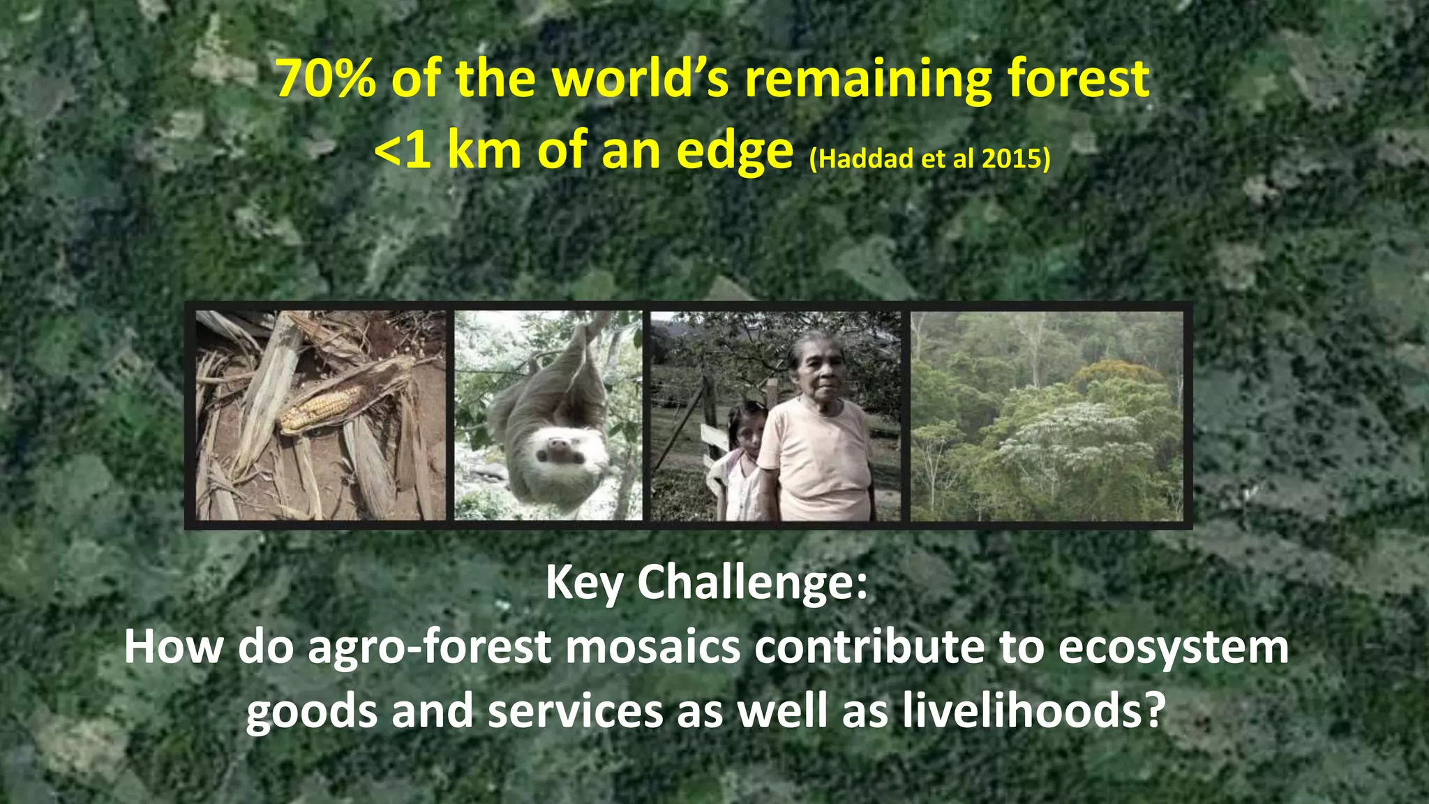

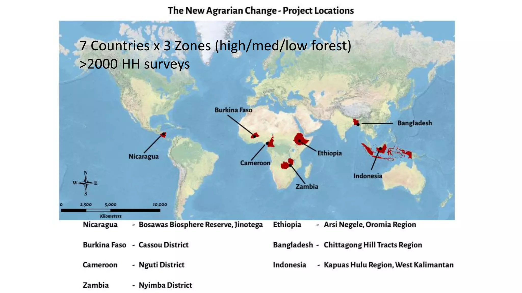
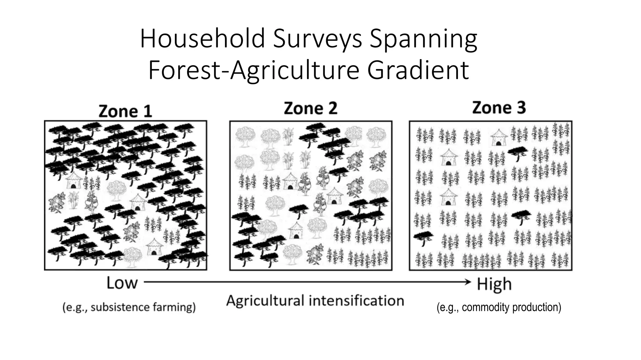
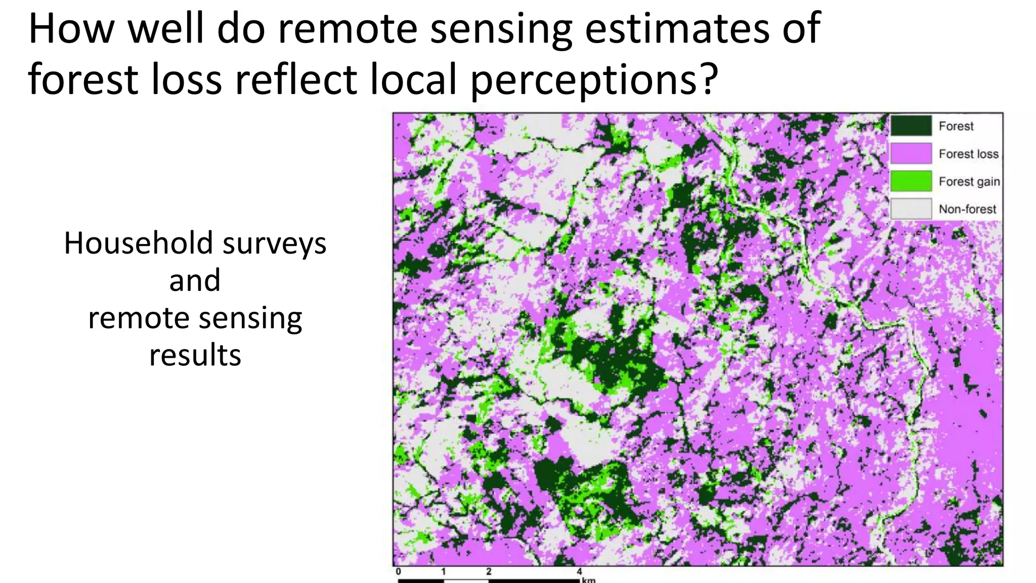
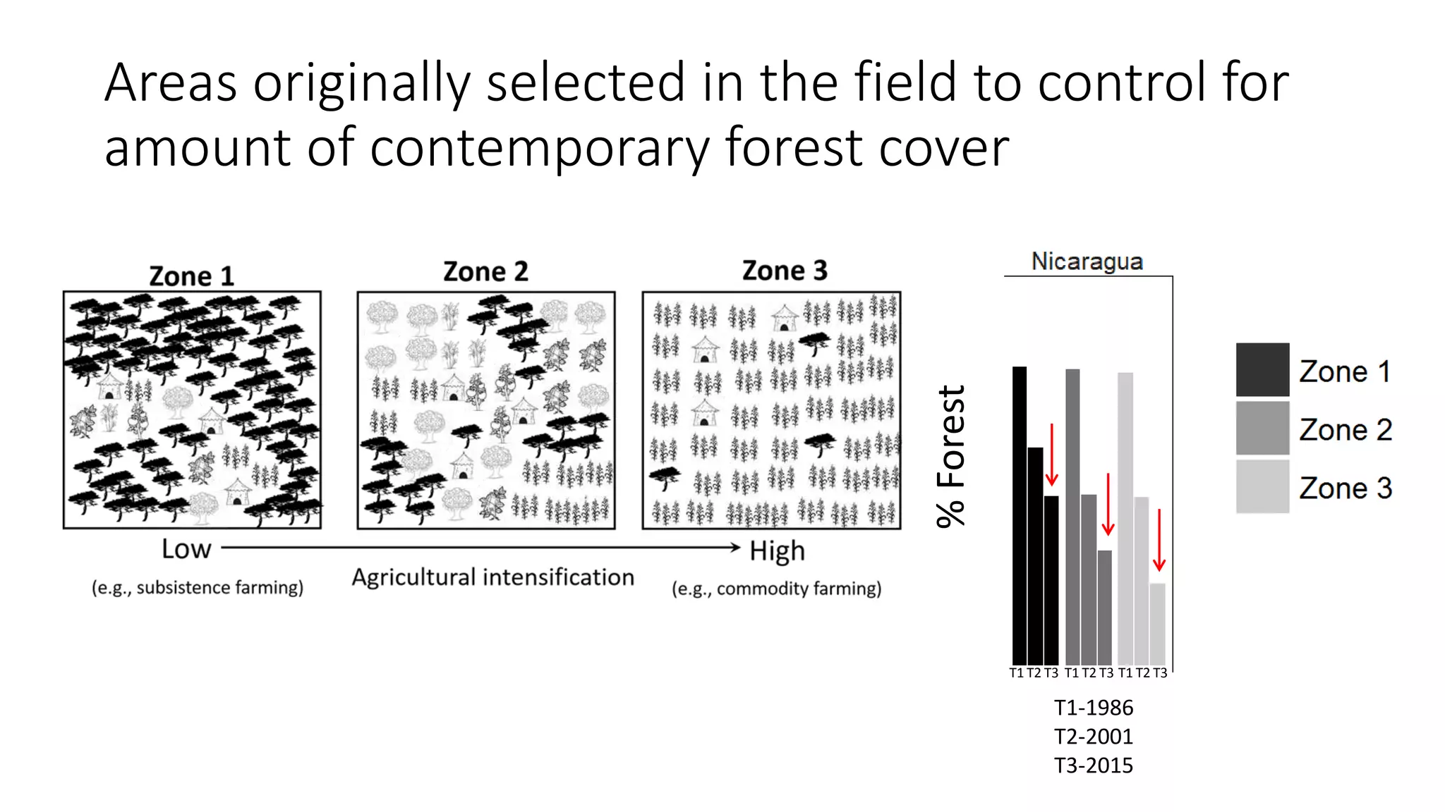
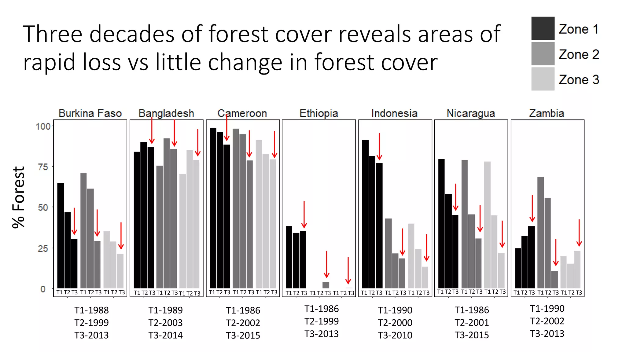
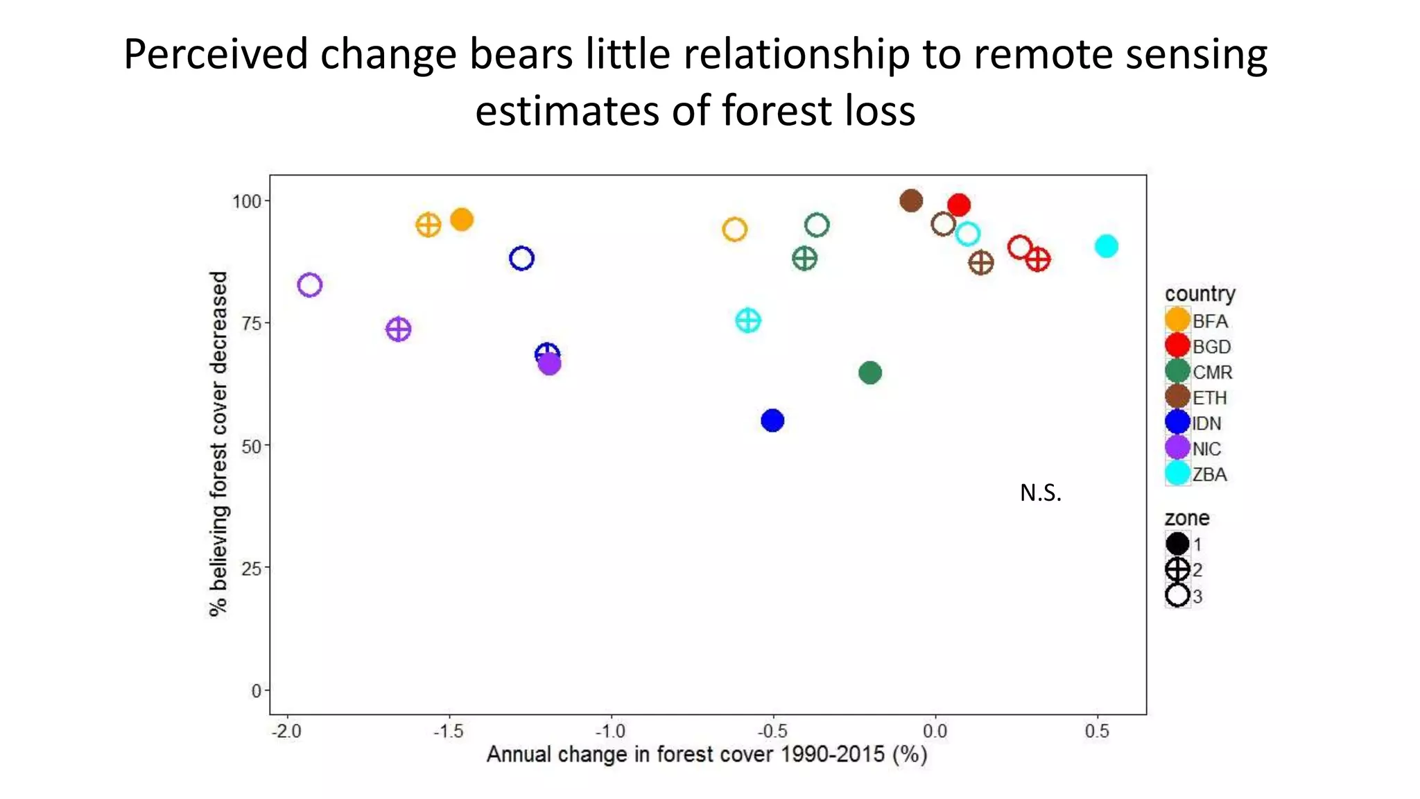
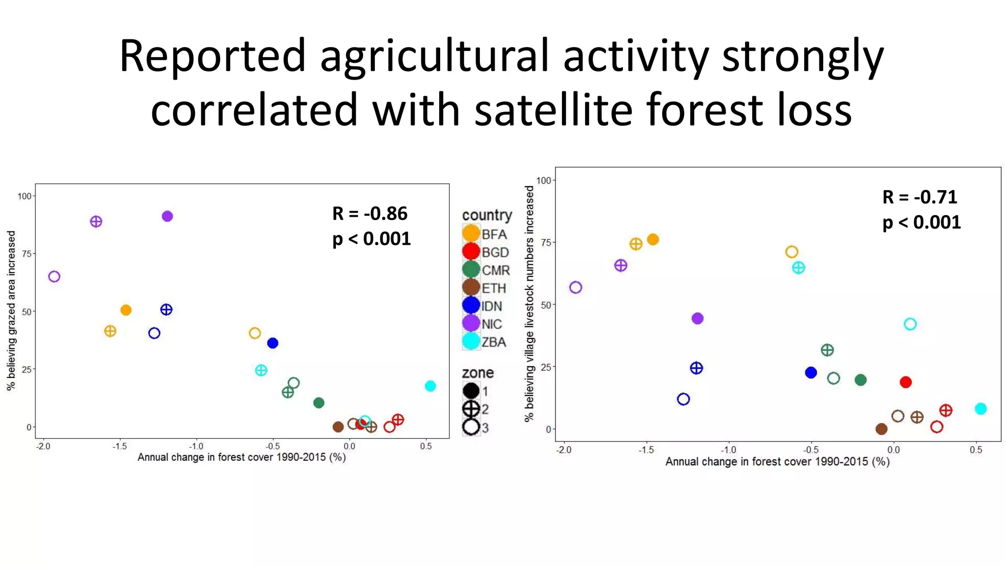
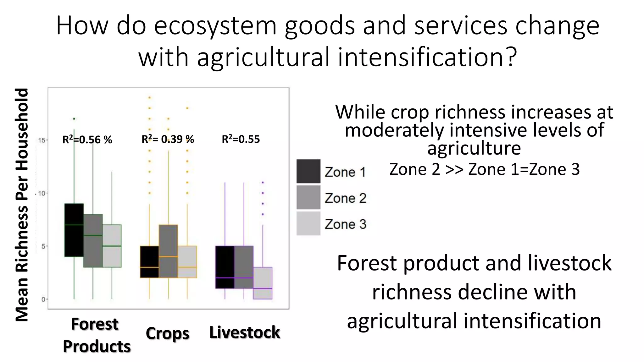
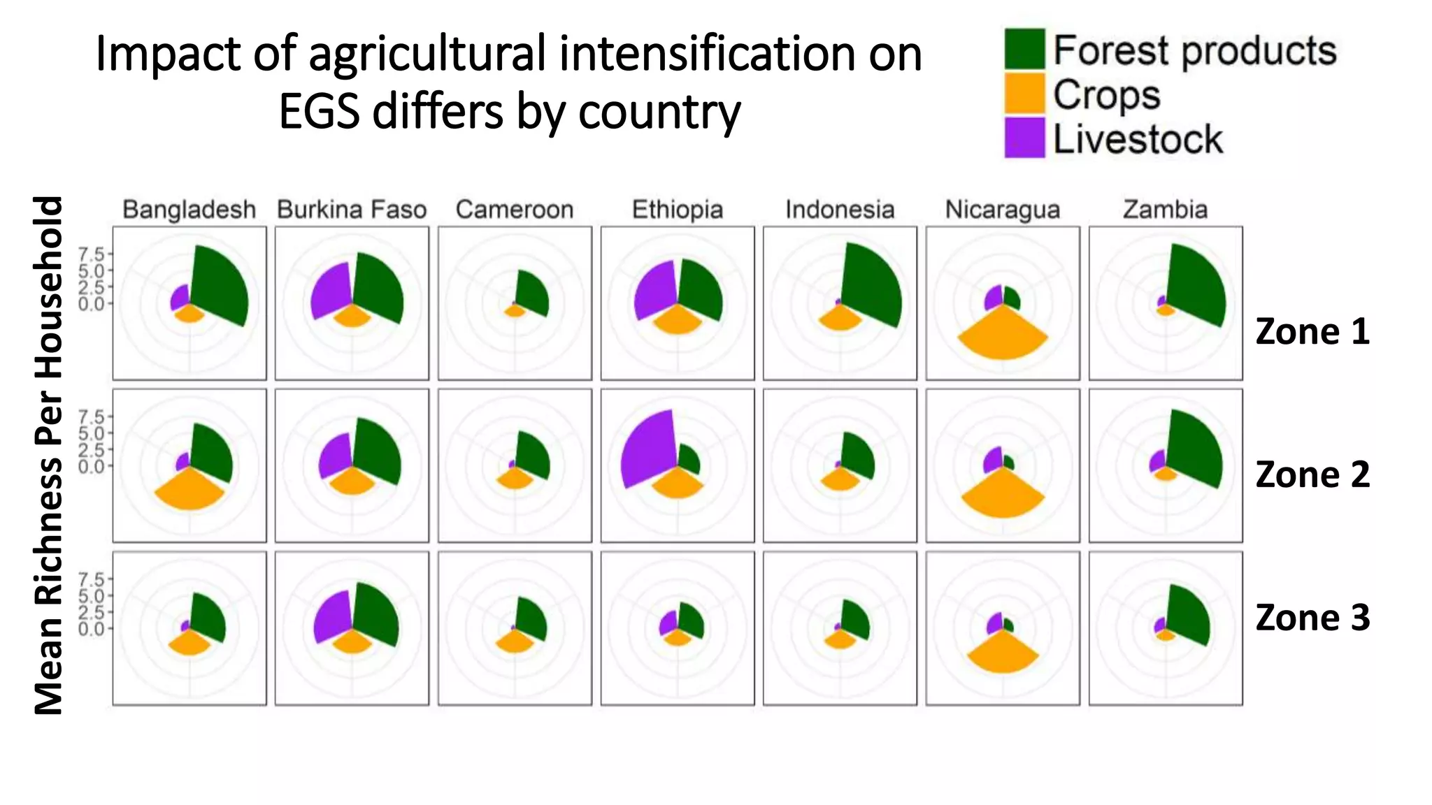
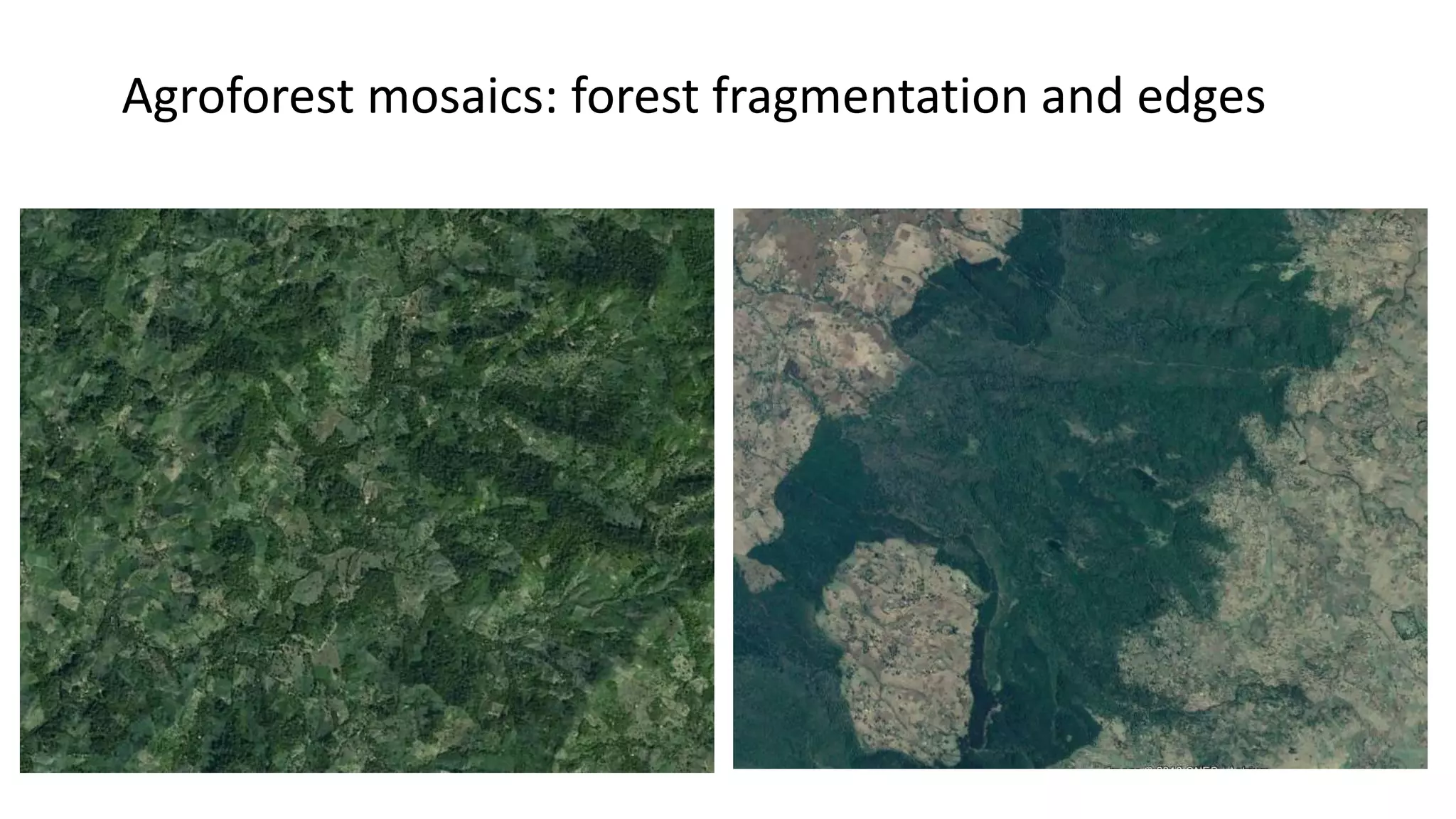
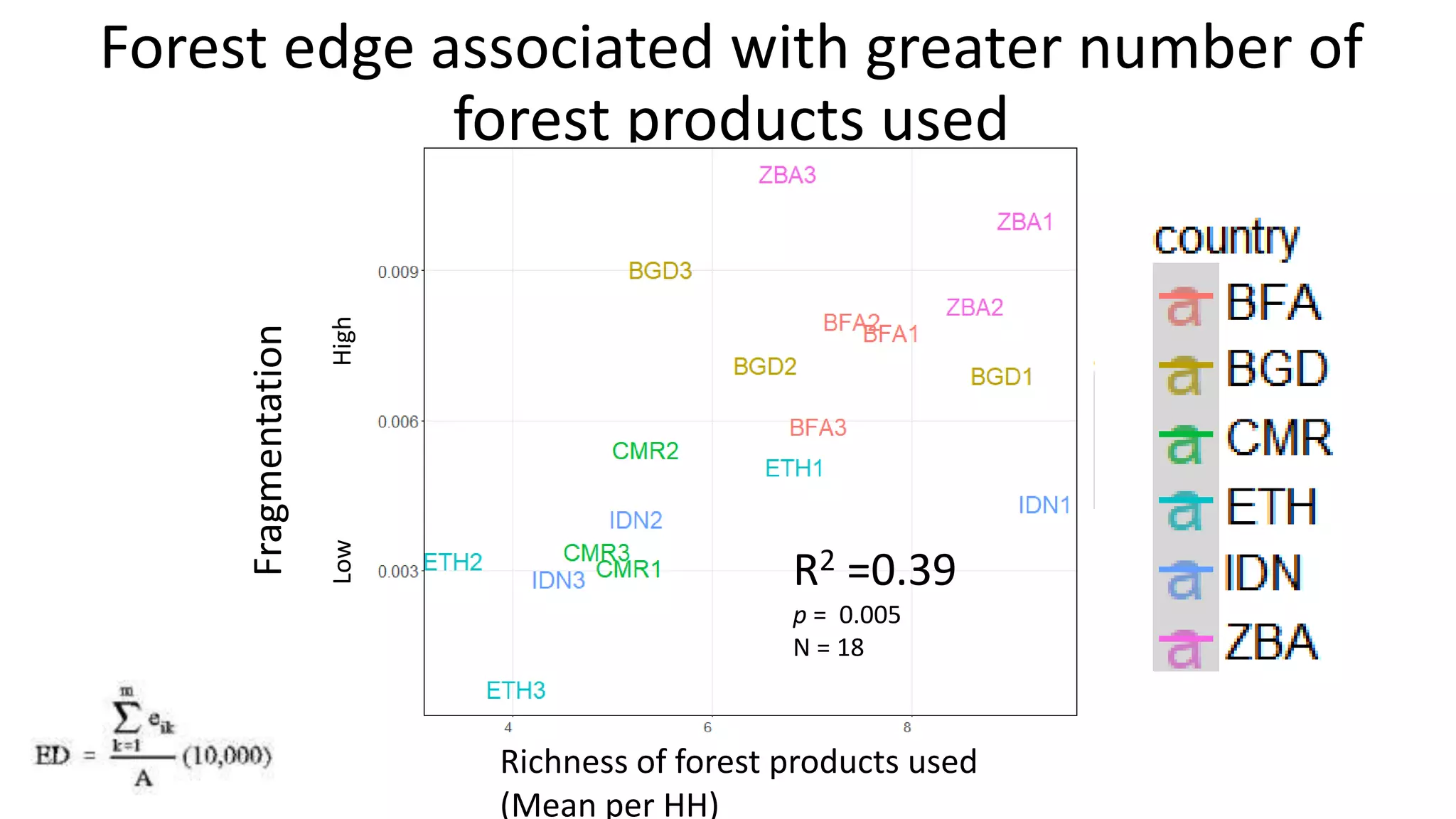
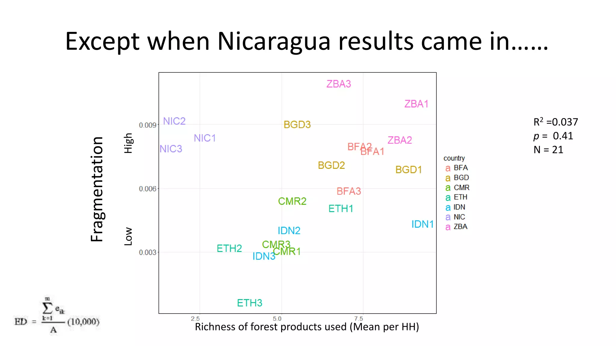
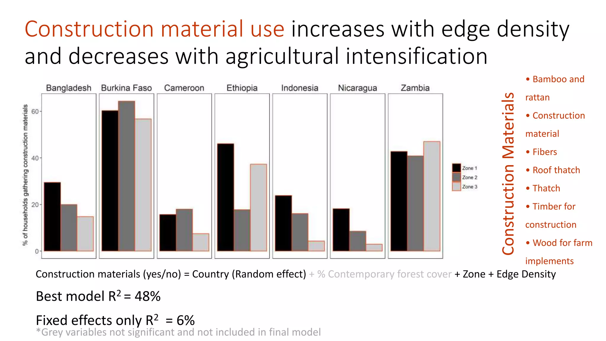
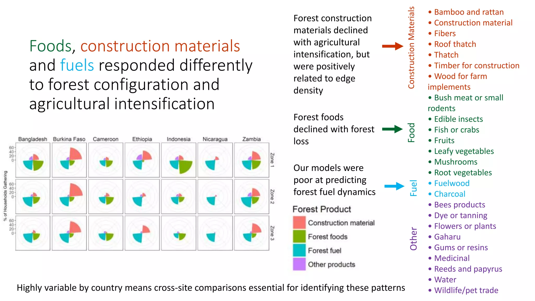
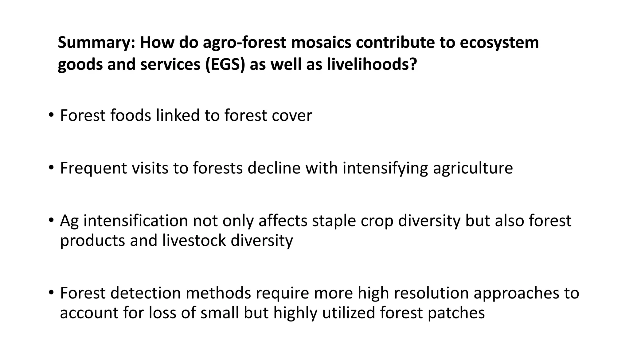


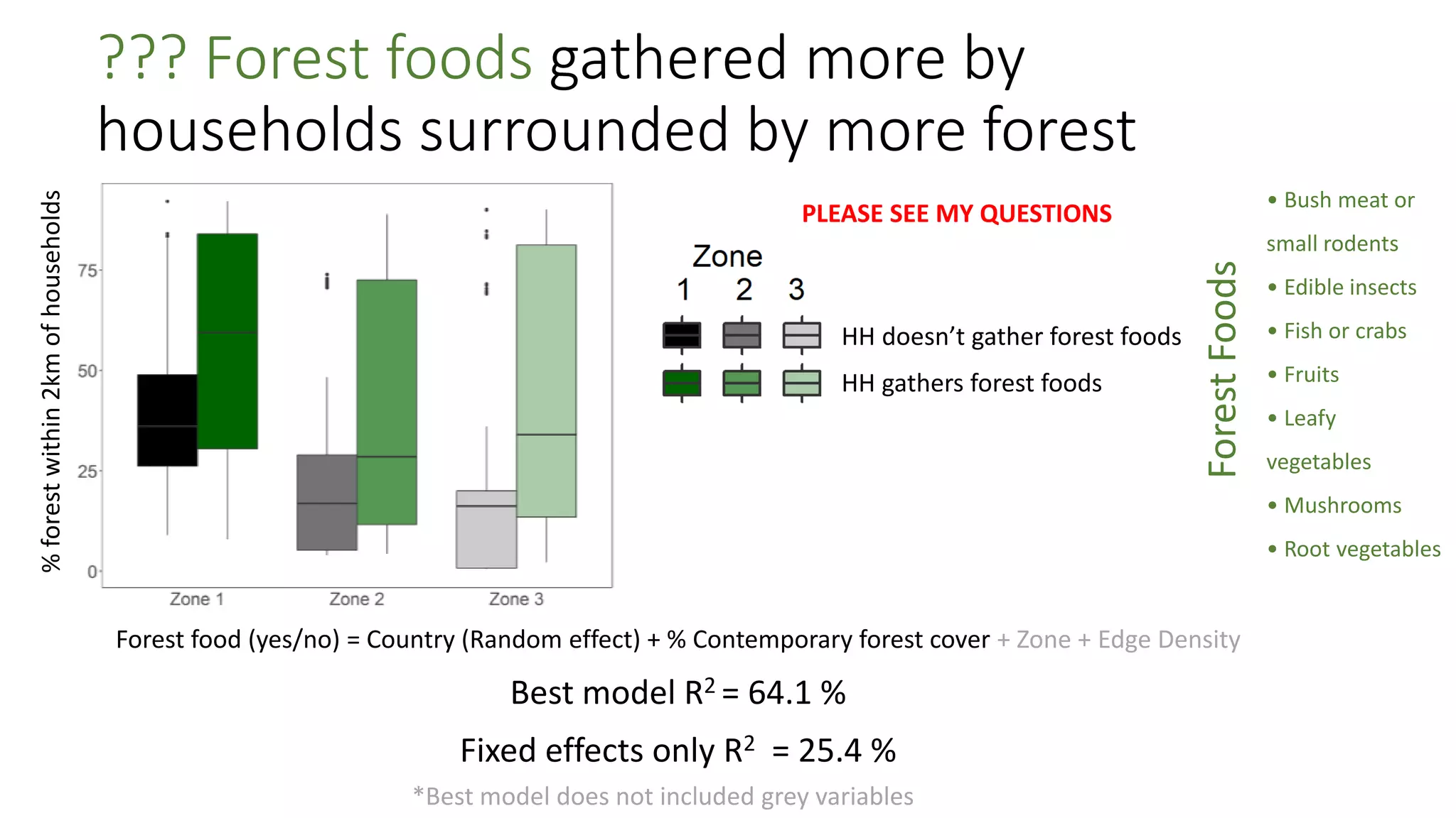
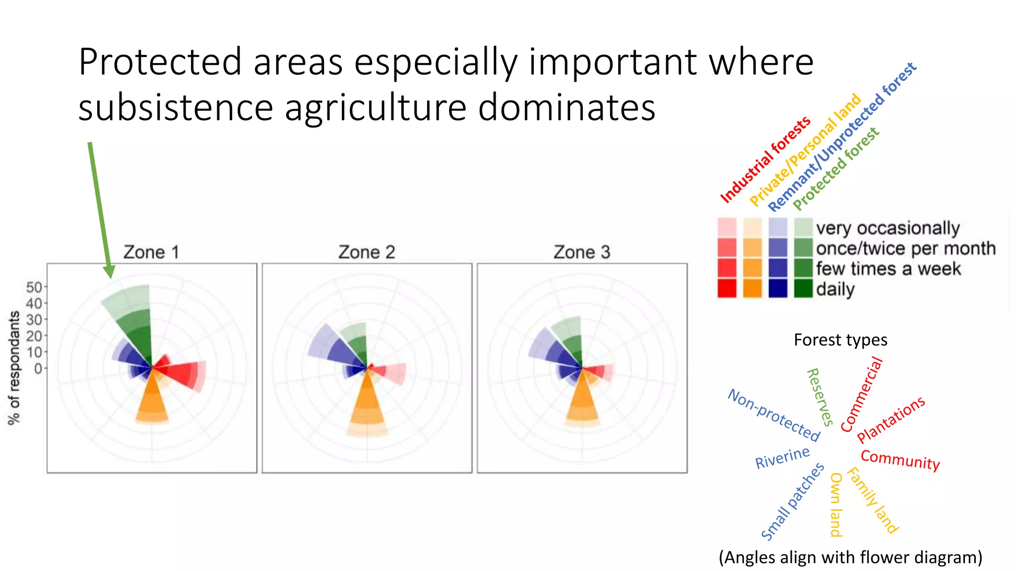
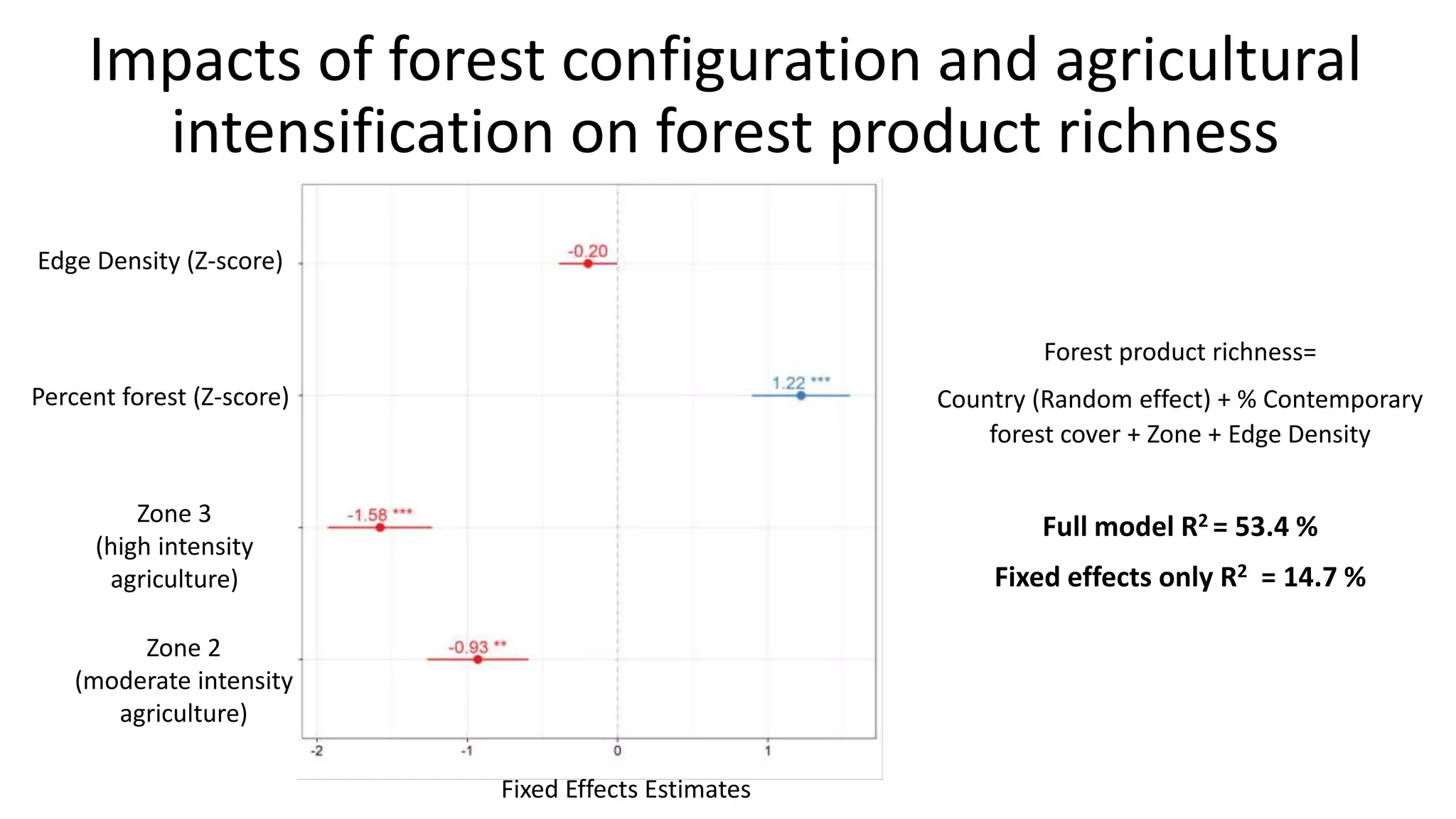
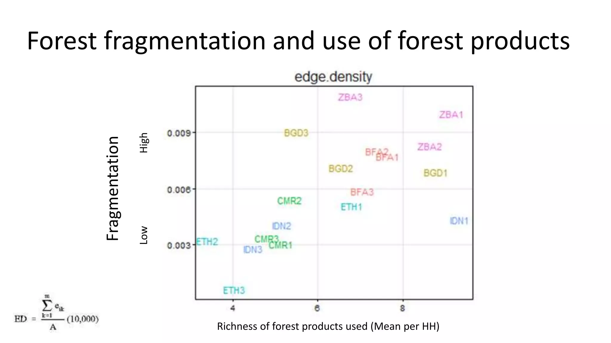
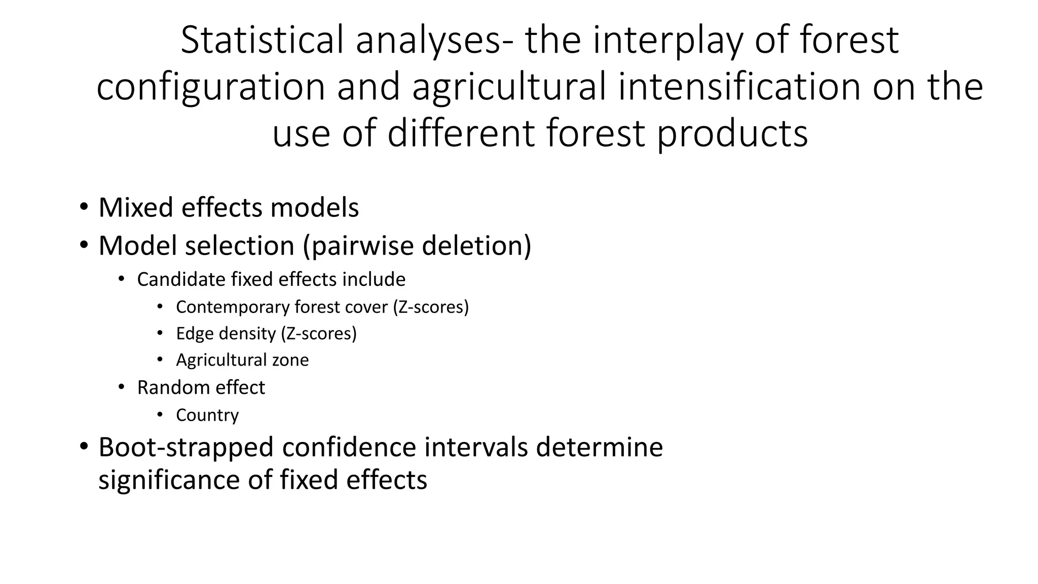

The document examines the interaction between forest loss, fragmentation, and agricultural intensification across seven countries, focusing on how agro-forest mosaics influence ecosystem goods and services as well as local livelihoods. Key findings indicate that agricultural intensification correlates with decreased visits to forests, lower biodiversity in forest products, and a disparity between local perceptions of forest loss and remote sensing data. The study emphasizes the importance of high-resolution forest detection methods and cross-site comparisons to understand these dynamics better.


