1. ADCIRC Model and Static / Dynamic Method
Mapping Static and Dynamic Models of Sea Level Rise Enhanced Tidal Inundation Along Florida's Northern and Central Atlantic Coast
Brandon S. Dees1, Sandra Fox2, and Ed Carter2. St. John’s River Water Management District (SJRWMD), P.O. Box 1429, Palatka, Florida 32178
SJRWMD contracted with UCF Coastal Hydroscience Analysis, Modeling &
Predictive Simulations Laboratory to quantify the extent to which sea level rise
(SLR) could reasonably be expected to enhance inundation of coastal areas in
extreme events such as hurricanes, as well as through nominal astronomical
tides. The increases in sea level that were modeled are based on projected
U.S. Army Corps of Engineers (USACE) values using both a static (“bathtub”)
method and a dynamic method: 0.13 m, 0.22 m, 0.25 m, 0.51 m, 0.56 m and
1.57 m. (Hagen, Wang, et al. 2014.)
Figure 1. Chart taken from the 2014 UCF report showing predicted SLR
scenarios by NOAA and USACE, based on a linear extrapolation of tide gauge
readings at Mayport Ferry Depot.
Table 1. USACE
SLR scenarios at
Mayport, FL from
highest to lowest
(Hagen, Wang, et al.
2014.)
Scenario Name Case Number
Sea Level Rise
(m)*
1992 0 0
2050 Low 1 0.13
2050 Intermediate 2 0.22
2050 High 3 0.51
2100 Low 4 0.25
2100 Intermediate 5 0.56
2100 High 6 1.57
Additional parameters are modified to account
for effects of the inundation interaction with
coastal floodplains, and the simulation is run as
previously described.
A total of twelve shapefiles were delivered by
UCF. These polyline shapefiles represented the
inundation extents of both static and dynamic
methods for the six inundation scenarios
projected by USACE. In several areas of interest
within the SJRWMD, the UCF team found that the
static method generally produced additional
inundation area than were produced with the
dynamic simulations.
SJRWMD Geospatial Processing and Analysis
The twelve product polyline shapefiles were edited by GIS staff at SJRWMD to create areas, facilitating
construction of inundation polygon features. These features were edited to remove polygon features
representing “dry” areas for each inundation scenario. Finally, the smaller component polygon features
were then merged to create a single feature coverage for each inundation scenario.
District GIS staff then used the SJRWMD Spatial Data Summary Tool to summarize the area of each Land
Use class within the District that would be inundated under each scenario.
All features within the Florida Land Use Land Cover Classification System (FLUCCS) series for water
(which is assumed as presently inundated) were removed from the 2009 SJRWMD Land Use input layer.
Using the inundation polygon for each scenario as the "area of interest" layer, the SJRWMD Spatial Data
Summary Tool clips the land use features inside the inundation polygon. This process produced a tabular
summary of estimated inundation impact for each land use class and a product geodatabase feature class of
inundated land use for each inundation scenario. From multiple iterations of this process, District staff
produced a master summary table with the predicted inundated acreage of each land use feature for all
twelve inundation scenarios.
SJRWMD Spatial
Data Summary Tool
Conclusion and Discussion
Table 2. Table compiled from SJRWMD Spatial Data Summary Tool output.
Figure 5. Map of 2009
SJRWMD Inundated Land Use.
Product dataset of processing
through SJRWMD Spatial Data
Summary Tool.
Figure 3. Comparison of static vs. dynamic inundation
extents for a given SLR scenario. The twelve polyline
extent shapefiles were processed to create mask
polygon features which served as the AOI in the
SJRWMD Spatial Data Summary Tool process.
Figure 4. 2009 SJRWMD Land Use coverage.
A similar coverage with water features
omitted was used as the input layer for
SJRWMD Spatial Data Summary Tool
processing. Figures 6-9. Graphics created from Table 2 depicting relative effects of inundation on wetlands vs. non-wetland features and
detailed effects on non-wetland features in the Case 5 inundation scenario.
Wetlands generally appear to be most vulnerable to inundation due to predicted SLR in all scenarios. However, a significant amount of non-
wetland acreage will also be affected, even in the most conservative estimates.
EST INUNDATION IMPACT
Inundation Scenarios
Case 1 (+0.13m SLR) Case 2 (+0.22m SLR) Case 3 (+0.51m SLR) Case 4 (+0.25m SLR) Case 5 (+0.56m SLR) Case 6 (+1.57m SLR)
Static Dynamic Static Dynamic Static Dynamic Static Dynamic Static Dynamic Static Dynamic
2009 Detailed SJRWMD Land Use Acreage Acreage Acreage Acreage Acreage Acreage Acreage Acreage Acreage Acreage Acreage Acreage
Residential 3213 2882 3348 2997 4532 3858 3397 3036 4961 4028 30984 23212
Commercial 124 101 127 104 154 139 129 106 169 143 2468 1802
Industrial 29 28 32 29 53 41 34 29 56 46 448 354
Extractive 63 42 90 59 137 115 91 59 139 116 177 173
Institutional 59 55 63 66 125 94 71 71 162 100 5208 2111
Recreation 1809 1677 1904 1744 2401 2136 1935 1783 2532 2226 6446 5312
Open land 44 21 44 23 52 49 44 39 78 51 558 463
Agriculture 224 138 251 193 433 338 263 227 586 401 12982 11684
Upland nonforested 961 588 1088 820 1842 1393 1133 920 2062 1554 23888 15004
Coniferous forest 435 377 515 408 1187 700 545 418 1353 798 6044 5119
Hardwood forest 2388 1983 2595 2176 3720 3058 2667 2265 4100 3255 21817 15776
Tree plantation 131 40 182 81 584 174 203 86 753 206 6650 4815
Hardwood forested wetland 24190 11994 40295 18493 77494 66702 46038 22005 81862 72169 129223 124370
Coniferous forested wetland 758 230 1555 388 6657 4876 2852 537 7111 5676 14280 13954
Mixed forested wetland 1383 598 1633 733 4027 2879 1759 804 4678 3351 19976 17210
Nonforested wetland 80937 69721 87048 77200 109986 99732 88709 79599 113400 105352 163011 159013
Nonvegetated wetland 2136 1887 2233 2113 2473 2480 2268 2151 2494 2508 3178 3148
Barren land 191 139 250 187 410 373 271 200 439 402 1053 982
Transportation, Communication, Utilities 231 199 253 208 351 288 263 211 372 304 3042 1765
Figure 2. Slide from UCF report with ADCIRC mesh detail of the Lower St. John’s River Basin (Hagen, Wang, et al. 2014) The amount of affected Residential area begins to show a moderate increase beginning in the high 2050 / intermediate 2100 predicted SLR of
0.5 – 0.56m. In addition, breaching and significant inundation begin to occur on the barrier islands in the intermediate and high 2100 prediction
scenarios.
• Although Sea Level Rise will enhance tidal inundation and significantly impact natural features, anthropocentric features
will be affected as well.
• Using a similar methodology, SJRWMD can use future Land Use datasets as they become available to perform analyses
and predict trends of the potential impacts of Sea Level Rise to core District functions.
Credits
Sandra Fox, M.S., GISP
Ed Carter, Hydrologist III
Brandon S. Dees, MSGIS
The ADvanced CIRCulation Model
(ADCIRC) is a hydrodynamic
circulation model used by federal
agencies and academia to model tidal,
wind, and wave-driven circulation in
coastal waters.
For the purposes of this study, the
static method entails taking each
node of the maximum water surface
elevation previously calculated by
ADCIRC simulation for the current
sea level (i.e., adjusted with a geoid
offset for elevation obtained from a
NOAA tide gauge and based from
the 1992 tidal epoch that NOAA
utilizes), and adding the specified
SLR magnitude across the study
area.
If a node adjacent to a "wet" node was
designated "dry" (i.e., node elevation
value > MSL) in the current sea level
mesh, it is checked to see if its value is
less than the new computed maximum
water surface elevation. If it is, it will
be designated as "wet“ in the new
model output.
This process is reiterated until the
process results in zero node status
changes.
The dynamic method is meant to more
closely depict the influence of
astronomic tide-generated flow.
However, the SLR magnitude for the
scenario is included within the geoid
offset parameter of the model.