This paper talks about optimization algorithms used for big data applications. We start with explaining the gradient descent algorithms and its limitations. Later we delve into the stochastic gradient descent algorithms and explore methods to improve it it by adjusting learning rates.

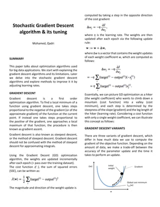
1. Stochastic Gradient Descent
algorithm & its tuning
Mohamed, Qadri
SUMMARY
This paper talks about optimization algorithms used
for big data applications. We start with explaining the
gradient descent algorithms and its limitations. Later
we delve into the stochastic gradient descent
algorithms and explore methods to improve it it by
adjusting learning rates.
GRADIENT DESCENT
Gradient descent is a first order
optimization algorithm. To find a local minimum of a
function using gradient descent, one takes steps
proportional to the negative of the gradient (or of the
approximate gradient) of the function at the current
point. If instead one takes steps proportional to
the positive of the gradient, one approaches a local
maximum of that function; the procedure is then
known as gradient ascent.
Gradient descent is also known as steepest descent,
or the method of steepest descent. Gradient descent
should not be confused with the method of steepest
descent for approximating integrals.
Using the Gradient Decent (GD) optimization
algorithm, the weights are updated incrementally
after each epoch (= pass over the training dataset).
The cost function J(⋅), the sum of squared errors
(SSE), can be written as:
The magnitude and direction of the weight update is
computed by taking a step in the opposite direction
of the cost gradient
where η is the learning rate. The weights are then
updated after each epoch via the following update
rule:
where Δw is a vector that contains the weight updates
of each weight coefficient w, which are computed as
follows:
Essentially, we can picture GD optimization as a hiker
(the weight coefficient) who wants to climb down a
mountain (cost function) into a valley (cost
minimum), and each step is determined by the
steepness of the slope (gradient) and the leg length of
the hiker (learning rate). Considering a cost function
with only a single weight coefficient, we can illustrate
this concept as follows:
GRADIENT DESCENT VARIANTS
There are three variants of gradient descent, which
differ in how much data we use to compute the
gradient of the objective function. Depending on the
amount of data, we make a trade-off between the
accuracy of the parameter update and the time it
takes to perform an update.

2. Batch Gradient Descent
Vanilla gradient descent, aka batch gradient descent,
computes the gradient of the cost function w.r.t. to
the parameters θ for the entire training dataset:
As we need to calculate the gradients for the whole
dataset to perform just one update, batch gradient
descent can be very slow and is intractable for
datasets that don't fit in memory. Batch gradient
descent also doesn't allow us to update our
model online, i.e. with new examples on-the-fly.
In code, batch gradient descent looks something like
this:
for i in range(nb_epochs):
params_grad =
evaluate_gradient(loss_function,
data, params)
params = params - learning_rate *
params_grad
For a pre-defined number of epochs, we first
compute the gradient vector weights_grad of
the loss function for the whole dataset w.r.t. our
parameter vector params. We then update our
parameters in the direction of the gradients with the
learning rate determining how big of an update we
perform. Batch gradient descent is guaranteed to
converge to the global minimum for convex error
surfaces and to a local minimum for non-convex
surfaces.
Stochastic Gradient Descent
Stochastic gradient descent (SGD) in contrast
performs a parameter update for each training
example x(i)x(i)and label y(i)y(i):
θ=θ−η⋅∇θJ(θ;x(i);y(i))
Batch gradient descent performs redundant
computations for large datasets, as it recomputes
gradients for similar examples before each parameter
update. SGD does away with this redundancy by
performing one update at a time. It is therefore
usually much faster and can also be used to learn
online.
SGD performs frequent updates with a high variance
that cause the objective function to fluctuate heavily
as in Image.
While batch gradient descent converges to the
minimum of the basin the parameters are placed in,
SGD's fluctuation, on the one hand, enables it to jump
to new and potentially better local minima. On the
other hand, this ultimately complicates convergence
to the exact minimum, as SGD will keep overshooting.
However, it has been shown that when we slowly
decrease the learning rate, SGD shows the same
convergence behavior as batch gradient descent,
almost certainly converging to a local or the global
minimum for non-convex and convex optimization
respectively.
Its code fragment simply adds a loop over the training
examples and evaluates the gradient w.r.t. each
example.
for i in range(nb_epochs):
np.random.shuffle(data)
for example in data:
params_grad =
evaluate_gradient(loss_function,
example, params)
params = params - learning_rate
* params_grad
In both gradient descent (GD) and stochastic gradient
descent (SGD), you update a set of parameters in an
iterative manner to minimize an error function.
While in GD, you have to run through ALL the samples
in your training set to do a single update for a
parameter in a particular iteration, in SGD, on the
other hand, you use ONLY ONE training sample from
your training set to do the update for a parameter in
a particular iteration.
Thus, if the number of training samples are large, in
fact very large, then using gradient descent may take
too long because in every iteration when you are
updating the values of the parameters, you are
running through the complete training set. On the

3. other hand, using SGD will be faster because you use
only one training sample and it starts improving itself
right away from the first sample.
SGD often converges much faster compared to GD
but the error function is not as well minimized as in
the case of GD. Often in most cases, the close
approximation that you get in SGD for the parameter
values are enough because they reach the optimal
values and keep oscillating there.
There are several different flavors of SGD, which can
be all seen throughout literature. Let's take a look at
the three most common variants:
A)
• randomly shuffle samples in the training set
• for one or more epochs, or until approx. cost
minimum is reached
• for training sample i
• compute gradients and perform weight updates
B)
• for one or more epochs, or until approx. cost
minimum is reached
• randomly shuffle samples in the training set
• for training sample i
• compute gradients and perform weight updates
C)
• for iterations t, or until approx. cost minimum is
reached:
• draw random sample from the training set
• compute gradients and perform weight updates
In scenario A , we shuffle the training set only one
time in the beginning; whereas in scenario B, we
shuffle the training set after each epoch to prevent
repeating update cycles. In both scenario A and
scenario B, each training sample is only used once per
epoch to update the model weights.
In scenario C, we draw the training samples randomly
with replacement from the training set. If the number
of iterations t is equal to the number of training
samples, we learn the model based on a bootstrap
sample of the training set.
In the Gradient Descent method, one computes the
direction that decreases the objective function the
most in the case of minimization problems. But
sometimes this cant be quite costly. In most Machine
Learning for example, the objective function is often
the cumulative sum of the error over the training
examples. But the size of the training examples set
might be very large and hence computing the actual
gradient would be computationally expensive.
In Stochastic Gradient (Descent) method, we
compute an estimate or approximation to this
direction. The most simple way is to just look at one
training example (or subset of training examples) and
compute the direction to move only on this
approximation. It is called as Stochastic because the
approximate direction that is computed at every step
can be thought of a random variable of a stochastic
process. This is mainly used in showing the
convergence of this algorithm.
Recent theoretical results, however, show that the
runtime to get some desired optimization accuracy
does not increase as the training set size increases.
Stochastic Gradient Descent is sensitive to feature
scaling, so it is highly recommended to scale your
data. For example, scale each attribute on the input
vector X to [0,1] or [-1,+1], or standardize it to have
mean 0 and variance 1. Note that the same scaling
must be applied to the test vector to obtain
meaningful results.
Empirically, we found that SGD converges after
observing approx. 10^6 training samples. Thus, a
reasonable first guess for the number of iterations
is n_iter = np.ceil(10**6 / n), where n is the size of the
training set.
If you apply SGD to features extracted using PCA we
found that it is often wise to scale the feature values
by some constant c such that the average L2 norm of
the training data equals one.
We found that Averaged SGD works best with a larger
number of features and a higher eta0
Here, the term "stochastic" comes from the fact that
the gradient based on a single training sample is a
"stochastic approximation" of the "true" cost

4. gradient. Due to its stochastic nature, the path
towards the global cost minimum is not "direct" as in
GD, but may go "zig-zag" if we are visualizing the cost
surface in a 2D space. However, it has been shown
that SGD almost surely converges to the global cost
minimum if the cost function is convex (or pseudo-
convex).
There might be many reason but one reason as to why
SG is preferred in Machine Learning is because it
helps the algorithm to skip some local minima.
Though this is not a theoretically sound reason in my
opinion, the optimal points that are computed using
SG are empirically better than the GD method often.
SGD is just one type of online learning
algorithm. There are many other online learning
algorithms that may not depend on gradients (e.g.
perceptron algorithm, bayesian inference, etc).
Mini-Batch Gradient Descent
Mini-batch gradient descent finally takes the best of
both worlds and performs an update for every mini-
batch of n training examples:
θ=θ−η⋅∇θJ(θ;x(i:i+n);y(i:i+n))
This way, it a) reduces the variance of the parameter
updates, which can lead to more stable convergence;
and b) can make use of highly optimized matrix
optimizations common to state-of-the-art deep
learning libraries that make computing the gradient
w.r.t. a mini-batch very efficient. Common mini-batch
sizes range between 50 and 256, but can vary for
different applications. Mini-batch gradient descent is
typically the algorithm of choice when training a
neural network and the term SGD usually is employed
also when mini-batches are used. Note: In
modifications of SGD in the rest of this post, we leave
out the parameters x(i:i+n);y(i:i+n)x(i:i+n);y(i:i+n) for
simplicity.
Challenges
Vanilla mini-batch gradient descent, however, does
not guarantee good convergence, but offers a few
challenges that need to be addressed:
Choosing a proper learning rate can be difficult. A
learning rate that is too small leads to painfully slow
convergence, while a learning rate that is too large
can hinder convergence and cause the loss function
to fluctuate around the minimum or even to diverge.
Learning rate schedules try to adjust the learning rate
during training by e.g. annealing, i.e. reducing the
learning rate according to a pre-defined schedule or
when the change in objective between epochs falls
below a threshold. These schedules and thresholds,
however, have to be defined in advance and are thus
unable to adapt to a dataset's characteristics.
Additionally, the same learning rate applies to all
parameter updates. If our data is sparse and our
features have very different frequencies, we might
not want to update all of them to the same extent,
but perform a larger update for rarely occurring
features.
Another key challenge of minimizing highly non-
convex error functions common for neural networks
is avoiding getting trapped in their numerous
suboptimal local minima. Some scientists argue that
the difficulty arises in fact not from local minima but
from saddle points, i.e. points where one dimension
slopes up and another slopes down. These saddle
points are usually surrounded by a plateau of the
same error, which makes it notoriously hard for SGD
to escape, as the gradient is close to zero in all
dimensions.
There are some algorithms that are widely used by
the deep learning community to deal with the
aforementioned challenges. Below are some of
them.
Momentum
SGD has trouble navigating ravines, i.e. areas where
the surface curves much more steeply in one
dimension than in another, which are common
around local optima. In these scenarios, SGD
oscillates across the slopes of the ravine while only
making hesitant progress along the bottom towards
the local optimum as in Image 2.

5. 2: SGD without momentum
3: SGD with momentum
Momentum is a method that helps accelerate SGD in
the relevant direction and dampens oscillations as
can be seen in Image 3. It does this by adding a
fraction γ of the update vector of the past time step
to the current update vector:
Essentially, when using momentum, we push a ball
down a hill. The ball accumulates momentum as it
rolls downhill, becoming faster and faster on the way
(until it reaches its terminal velocity if there is air
resistance, i.e. γ<1). The same thing happens to our
parameter updates: The momentum term increases
for dimensions whose gradients point in the same
directions and reduces updates for dimensions whose
gradients change directions. As a result, we gain
faster convergence and reduced oscillation.
Nesterov Accelerated Gradient
However, a ball that rolls down a hill, blindly following
the slope, is highly unsatisfactory. We'd like to have a
smarter ball, a ball that has a notion of where it is
going so that it knows to slow down before the hill
slopes up again.
Nesterov accelerated gradient (NAG) is a way to give
our momentum term this kind of prescience. We
know that we will use our momentum term γvt−1 to
move the parameters θ. Computing θ−γvt−1 thus gives
us an approximation of the next position of the
parameters (the gradient is missing for the full
update), a rough idea where our parameters are
going to be. We can now effectively look ahead by
calculating the gradient not w.r.t. to our current
parameters θ but w.r.t. the approximate future
position of our parameters:
Again, we set the momentum term γ to a value of
around 0.9. While Momentum first computes the
current gradient (small blue vector in Image 4) and
then takes a big jump in the direction of the updated
accumulated gradient (big blue vector), NAG first
makes a big jump in the direction of the previous
accumulated gradient (brown vector), measures the
gradient and then makes a correction (green vector).
This anticipatory update prevents us from going too
fast and results in increased responsiveness, which
has significantly increased the performance of RNNs
on a number of tasks.
Image 4
Adagrad
Adagrad is an algorithm for gradient-based
optimization that does just this: It adapts the learning
rate to the parameters, performing larger updates for
infrequent and smaller updates for frequent
parameters. For this reason, it is well-suited for
dealing with sparse data. Adagrad has greatly
improved the robustness of SGD and used it for
training large-scale neural nets at Google, which --
among other things -- learned to recognize cats in
YouTube videos.
Previously, we performed an update for all
parameters θ at once as every parameter θi used the
same learning rate η. As Adagrad uses a different
learning rate for every parameter θi at every time
step t, we first show Adagrad's per-parameter
update, which we then vectorize. For brevity, we
set gt,i to be the gradient of the objective function
w.r.t. to the parameter θi at time step t:
One of Adagrad's main benefits is that it eliminates
the need to manually tune the learning rate. Most
implementations use a default value of 0.01 and leave
it at that.
Adagrad's main weakness is its accumulation of the
squared gradients in the denominator: Since every
added term is positive, the accumulated sum keeps
growing during training. This in turn causes the

6. learning rate to shrink and eventually become
infinitesimally small, at which point the algorithm is
no longer able to acquire additional knowledge. The
following algorithms aim to resolve this flaw.
Adadelta
Adadelta is an extension of Adagrad that seeks to
reduce its aggressive, monotonically decreasing
learning rate. Instead of accumulating all past
squared gradients, Adadelta restricts the window of
accumulated past gradients to some fixed size w.
Instead of inefficiently storing w previous squared
gradients, the sum of gradients is recursively defined
as a decaying average of all past squared gradients.
The running average E[g2
]t at time step t then
depends (as a fraction γ similarly to the Momentum
term) only on the previous average and the current
gradient.
RMSprop
RMSprop is an unpublished, adaptive learning rate
method proposed by Geoff Hinton
RMSprop and Adadelta have both been developed
independently around the same time stemming from
the need to resolve Adagrad's radically diminishing
learning rates. RMSprop in fact is identical to the first
update vector of Adadelta that we derived above:
RMSprop as well divides the learning rate by an
exponentially decaying average of squared gradients.
Hinton suggests γ to be set to 0.9, while a good
default value for the learning rate η is 0.001.
Adam
Adaptive Moment Estimation (Adam) is another
method that computes adaptive learning rates for
each parameter. In addition to storing an
exponentially decaying average of past squared
gradients vt like Adadelta and RMSprop, Adam also
keeps an exponentially decaying average of past
gradients mt, similar to momentum:
mt=β1mt−1+(1−β1)gt
vt=β2vt−1+(1−β2)g2t
mt and vt are estimates of the first moment (the
mean) and the second moment (the uncentered
variance) of the gradients respectively, hence the
name of the method. As mt and vt are initialized as
vectors of 0's, the authors of Adam observe that they
are biased towards zero, especially during the initial
time steps, and especially when the decay rates are
small (i.e. β1 and β2 are close to 1).
ADDITIONAL STRATEGIES FOR OPTIMIZING SGD
Finally, we introduce additional strategies that can be
used alongside any of the previously mentioned
algorithms to further improve the performance of
SGD.
Shuffling And Curriculum Learning
Generally, we want to avoid providing the training
examples in a meaningful order to our model as this
may bias the optimization algorithm. Consequently, it
is often a good idea to shuffle the training data after
every epoch.
On the other hand, for some cases where we aim to
solve progressively harder problems, supplying the
training examples in a meaningful order may actually
lead to improved performance and better
convergence. The method for establishing this
meaningful order is called Curriculum Learning.
Batch Normalization
To facilitate learning, we typically normalize the initial
values of our parameters by initializing them with
zero mean and unit variance. As training progresses
and we update parameters to different extents, we
lose this normalization, which slows down training
and amplifies changes as the network becomes
deeper.
Batch normalization reestablishes these
normalizations for every mini-batch and changes are
back-propagated through the operation as well. By
making normalization part of the model architecture,

7. we are able to use higher learning rates and pay less
attention to the initialization parameters. Batch
normalization additionally acts as a regularizer,
reducing (and sometimes even eliminating) the need
for Dropout.
Early Stopping
You should thus always monitor error on a validation
set during training and stop (with some patience) if
your validation error does not improve enough.
Gradient Noise
Adding noise makes networks more robust to poor
initialization and helps training particularly deep and
complex networks. It is suspected that the added
noise gives the model more chances to escape and
find new local minima, which are more frequent for
deeper models.
We have then investigated algorithms that are most
commonly used for optimizing SGD: Momentum,
Nesterov accelerated gradient, Adagrad, Adadelta,
RMSprop, Adam, as well as different algorithms to
optimize asynchronous SGD. Finally, we've
considered other strategies to improve SGD such as
shuffling and curriculum learning, batch
normalization, and early stopping.
SGD has been successfully applied to large-scale and
sparse machine learning problems often encountered
in text classification and natural language processing.
Given that the data is sparse, the classifiers in this
module easily scale to problems with more than 10^5
training examples and more than 10^5 features.
Advantages of Stochastic Gradient Descent
• Efficiency.
• Ease of implementation (lots of opportunities for
code tuning).
Disadvantages of Stochastic Gradient Descent
• SGD requires a number of hyperparameters such
as the regularization parameter and the number
of iterations.
• SGD is sensitive to feature scaling.
• The class SGDClassifier in Sklearn implements a
plain stochastic gradient descent learning routine
which supports different loss functions and
penalties for classification.
• The class SGDRegressor implements a plain
stochastic gradient descent learning routine
which supports different loss functions and
penalties to fit linear regression
models. SGDRegressor is well suited for
regression problems with a large number of
training samples (> 10.000), for other problems
we recommend Ridge, Lasso, or ElasticNet.
The major advantage of SGD is its efficiency, which is
basically linear in the number of training examples. If
X is a matrix of size (n, p) training has a cost
of , where k is the number of iterations
(epochs) and is the average number of non-zero
attributes per sample.
Application
SGD algorithms can therefore be used in scenarios
where it is expensive to iterate over the entire dataset
several times. This algorithm is ideal for streaming
analytics, where we can discard the data after
processing it. We can use modified versions of SGD
such as mini batch GD etc, with adjusted learning
rates to get better results as seen above. This
algorithm can be used as the cost function of several
classification and regression techniques.
SGD in a real time scenario learns continuously as and
when the data comes in, somewhat like reinforced
machine learning using feedback. An example of this
can be a real time system where, it is judged on the
basis of some parameters, whether a customer is
genuine or not. Based on historical data the first set
of parameters are learnt. As a new customer comes
in with a new set of features, it falls into either of the
two groups : genuine, not genuine. Based on this
completed classification, the prior parameters of the
system are updated, using the features that the
customer brought in. Over time the system becomes
much smarter that what it started with. Apple’s Siri or
Microsoft’s Cortana assistants are also an example of
real time learning, which correct themselves on the
go.

8. Conclusion
In conclusion we saw that to manage large scale
data we can use variants of gradient descent, batch
gradient descent, stochastic gradient descent (SGD),
and mini gradient descent in the order of
improvement over the previous one. Each of which
differs in how much data we use to compute the
gradient of the objective function. Given the
ubiquity of large-scale data solutions and the
availability of low-commodity clusters, distributing
SGD to speed it up further is an obvious choice. SGD
by itself is inherently sequential: Step-by-step, we
progress further towards the minimum. Running it
provides good convergence but can be slow
particularly on large datasets. In contrast, running
SGD asynchronously is faster, but suboptimal
communication between workers can lead to poor
convergence. Additionally, we can also parallelize
SGD on one machine without the need for a large
computing cluster.
Depending on the amount of data, we make a trade-
off between the accuracy of the parameter update
and the time it takes to perform an update. To
overcome this challenge of parameter update using
the learning rate we looked at various methods that
address this problem such as momentum, Nesterov
Accelerated gradient, Adagrad, Adadelta, RMSProp
and Adam. In summary, RMSprop is an extension of
Adagrad that deals with its radically diminishing
learning rates. It is identical to Adadelta, except that
Adadelta uses the RMS of parameter updates in the
numinator update rule. Adam, finally, adds bias-
correction and momentum to RMSprop. Insofar,
RMSprop, Adadelta, and Adam are very similar
algorithms that do well in similar circumstances. Its
bias-correction helps Adam slightly outperform
RMSprop towards the end of optimization as
gradients become sparser. Insofar, Adam might be
the best overall choice.
Interestingly, many recent papers use vanilla SGD
without momentum and a simple learning rate
annealing schedule. As has been shown, SGD usually
achieves to find a minimum, but it might take
significantly longer than with some of the
optimizers, is much more reliant on a robust
initialization and annealing schedule, and may get
stuck in saddle points rather than local minima.
Consequently, if you care about fast convergence
and train a deep or complex neural network, you
should choose one of the adaptive learning rate
methods.
References
[1]Bottou, Léon (1998). "Online Algorithms and
Stochastic Approximations".
[2]Bottou, Léon. "Large-scale machine learning
with SGD."
[3]Bottou, Léon. "SGD tricks." Neural Networks:
Tricks of the Trade.
[4]https://www.quora.com/Whats-the-difference-
between-gradient-descent-and-stochastic-gradient-
descent
[5]http://ufldl.stanford.edu/tutorial/supervised/Op
timizationStochasticGradientDescent/
[6]http://scikit-learn.org/stable/modules/sgd.html
[7]http://sebastianruder.com/optimizing-gradient-
descent/