Fostering Friendships - Enhancing Social Bonds in the Classroom
4.3.2. controlling confounding stratification
1. 2014
Page
1
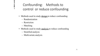
Confounding: Methods to
control or reduce confounding
• Methods used in study design to reduce confounding
– Randomization
– Restriction
– Matching
• Methods used in study analysis to reduce confounding
– Stratified analysis
– Multivariate analysis
31
2. • Basic goal of stratification is to evaluate the relationship
between the predictor (“cause”) and outcome (“effect”)
variable in strata homogenous with respect to potentially
confounding variables
40
3. 2014
Page
3
Confounding:The use of
stratification to reduce
confounding
• For example, to examine the relationship between smoking
and lung cancer while controlling for the potentially
confounding effect of gender:
– Create a 2x2 table (smoking vs. lung cancer) for men
and women separately
– To control for multiple confounders simultaneously,
stratify by pairs (or triplets or higher) of confounding
factors. For example, to control for gender and
race/ethnicity determine the OR for smoking vs. lung
cancer in multiple strata: white women, black
women, Hispanic women, white men, black men,
Hetics.panicmen, 41
4. 2014
Page
4
• (From the earlier example): Goal: create a summary or
“adjusted” estimate for the relationship between
matches and lung cancer while adjusting for the two
levels of smoking (the potential confounder)
• This process is analgous to the standardization of rates
earlier in the course—in those examples the purpose of
adjustment was to remove the confounding effect of age on
the relationship between populations (A vs. B etc.) and
rates of disease or death.
• In the present example the goal is to remove the
confounding effect of smoking on the relationship between
matches and lung cancer. 42
5. Confounding:Types of
summary estimators to
determine uniform effect
over strata• Mantel-Haenszel
– We will use this estimator in the present course
– Resistant to the effects of small strata or cells with a
value of “0”
– Computationally a piece of cake
• Directly pooled estimators (e.g. Woolf)
– Sensitive to small strata and cells with value “0”
– Computationally messy but doable
• Maximum likelihood
– The most “appropriate” estimator
– Resistant to the effects of small strata or cells with a
value of “0”
– Computationally
challenging
43
2014 Page 64
6. Confounding: smoking,
matches, and
lung cancer• ORpooled = 8.84 (7.2, 10.9)
• ORsmokers = 1.0 (0.6, 1.5)
• ORnonsmokers = 1.0 (0.5, 2.0)
Pooled Cancer No cancer
820
180
Cancer
810
340
660
No cancer
270
Matches No
Matches
Smokers
Matches
No Matches
Non-smoker
Matches
No Matches
2014
Page
6
90
Cancer
10
90
30
No cancer
70
630 44
7. 2014
Page
7 An
aside:
Termino
logy• Pooled = combined = collapsed = unadjusted
• Adjusted = summary = weighted, etc.
– All of these reflect some adjustment process such as
Mantel-Haenszel or Woolf or maximum likelihood
estimation to weight the strata and develop confidence
intervals about the estimate.
45
8. Confounding:Notation
used in Mantel-
Haenszel estimators of
relative risk
Case-control: RR = OR = ad / bc
Cohort: RR =
Ie
I0
46
a / (a + b)
=
c/ (c + d)
• Notation for case-control or cohort studies with count data
Cases Controls Total
2014
Page
8
a c b d a + b c + dExposed
Nonexposed
Total a + c b + d a + b + c + d = T
9. Confounding:Notation
used in Mantel- Haenszel
estimators of relative risk
(cont.)• Notation for cohort studies with person-time data
RR =
Ie
I0
=
a / PY1
2014
Page
9
47
c / PY0
Cases Controls
Exposed
Nonexposed
a c ---
---
PY1
PY0
Total a + c T
10. Confounding:Mantel-
Haenszel estimators of
relative risk for
stratified data
Case-Control Study:
RRMH =
∑(ad / T)
i
∑(bc / T)
i
Cohort Study with Count Denominators:
RRMH =
∑{a(c + d) / T}
i
∑{b(a + b) / T}I
Cohort Study with Person-years Denominators:
RRMH = ∑{a(PY ) / T}
0 i
∑{b(PY ) / T}
1 i
2014
Page
10
48
11. Confounding: smoking,
matches, and
lung cancer• ORpooled = 8.84 (7.2, 10.9)
• ORsmokers = 1.0 (0.6, 1.5)
•
No Matches
2014 Page 70
90 630 51
ORnonsmokers = 1.0 (0.5, 2.0)
Pooled Cancer No cancer
Matches 820 340
No Matches 180 660
Smokers Cancer No cancer
Matches 810 270
No Matches 90 30
Non-smoker Cancer No cancer
Matches 10 70
12. Confounding:Mantel-Haenszel estimators of
relative risk for stratified data (smoking, matches,
lung cancer
RRMH = ∑(ad / T)i / ∑(bc / T)i
Numerator of MH estimator:
• For smokers: (ad/T)=(810*30)/1200=20.25;
• For nonsmokers: (ad/T)=(10*630)/800=7.88;
• Add these together: 20.25 + 7.88=28.13 (numerator)
Denominator of MH estimator:
• For smokers: (bc/T)=(270*90)/1200=20.25;
• For nonsmokers: (bc/T)=(90*70)/800=7.88;
• Add these together: 20.25 + 7.88=28.13
•ORMH = 28.13 / 28.13 = 1.0 (as expected since both stratified OR’s were = 1.0)
•Be sure to try this on stratified data in which the two strata are not exactly equal
to each other (but also not so different as to suggest that effect modification is
present
52
2014
Page
12
13. Confounding:Interpretation of ORMH
• If ORMH (=1.0 in this example) “differs meaningfully”
from ORunadjusted (=8.8 in this example) then confounding is
present
• What does “differs meaningfully” mean
– This is a matter of judgment based on biologic/clinical
sense rather than on a statistical test
– Even if they “differ” only slightly, generally the ORMH
rather than the ORcombined is reported as the summary
effect estimate
• But what is one disadvantage of reporting ORMH ?
– Although there do exist statistical tests of confounding
they are not widely recommended (these tests evaluate53
2014
Page
13
Ho: OR = OR
MH unadjusted
20. • Confounding “pulls” the observed association away from the true
association
– It can either exaggerate/over-estimate the true association (positive
confounding)
• Example
– RRcausal = 1.0
–RRobserved = 3.0
or
– It can hide/under-estimate the true association (negative
confounding)
• Example
– RRcausal = 3.0
– RR = 1.0
observed
Direction of Confounding Bias
2014
Page
20
40
21. Confounding:Summary of
steps to evaluate
confounding
Table 12-10. Steps for the control of confounding and the evaluation of effect
modification through stratified analysis
1. Stratify by levels of the potential confounding factor.
2. Compute stratum-specific unconfounded relative risk estimates.
3. Evaluate similarity of the stratum-specific estimates by either eyeballing or
performing test of statistical significance. (More on this step later)
4. If the effect is thought to be uniform, calculate a pooled unconfounded summary
If effect is not uniform (i.e. effect modification is present,estimate using RRMH.
skip to step 6)
5. Perform hypothesis testing on the unconfounded estimate, using Mantel-Haenszel
chi-square and compute confidence interval.
6. If effect is not thought to be uniform (i.e., if effect modification is present):
a. Report stratum-specific estimates, results of hypothesis testing, and
confidence intervals for each estimate
b.If desired, calculate a summary unconfounded estimate using a standar6d6ized
formula 2014 Page 80