1. COMPUTER AIDED ENGINEERING – ANALYSIS
USING ANSYS- 14.0
EXPERIMENT-5
STRUCTURAL ANALYSIS OF 2-D TRUSS WITH INCLINED SUPPORT AND
SUPPORT SETTLEMENT
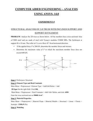
PROBLEM: Analyze the 2D truss as shown below. All the members have cross-sectional Area
of 5000 mm2 and are made of steel with Young’s modulus 210000 MPa. The Settlement at
support B is 10 mm. The roller at C is on a floor 45° from horizontal direction.
• If the applied force P is 200 kN, determine the member forces and stresses.
• Determine the maximum value of P in which the maximum member force does not
exceed 600 kN.
Step 1: Preferences: Structural
Step 2: Element Type and Real Constants
Main Menu > Preprocessor> Element Type > Add/Edit/Delete > Add
2D Spar 1in the right field. Click OK.
Main Menu > Preprocessor > Real Constants > Add/ Edit/ Delete, and click ADD
Enter the cross-sectional area as 5000E-6 m2
.
Step 3: Material Properties
Main Menu > Preprocessor > Material Props > Material Models > Structural > Linear > Elastic >
Isotropic >210Ee9 (Pa).
Step 4: Modeling
2. Main Menu > Preprocessor > Modeling > Create > Key points > In Active CS
Main Menu > Preprocessor > Modeling > Create > Lines > Lines >Straight Line
Step 5: Meshing
Main Menu > Preprocessor > Meshing > Mesh Tool
Step 6: Specify Boundary Conditions
Main Menu > Preprocessor > Loads > Define Loads > Apply > Structural > Displacement >On
Node. Now select point A and Select “ALL DOF” in the box showing DOF to be constrained. Next
Select point B and Constrain “UY” and set displacement value to -10e-3 m.
Work Plane > Local Coordinate Systems > Create Local CS > By 3 Nodes. Now Choose the nodes in
that order by clicking node 3, 5and 2, respectively (See figure below). Note that node 5 defines the
direction of the x-axis and node 2 defines the X-Y plane. Thedirection of y-axis is perpendicular to
the x-axis toward node 2. After you clicking the 3 nodes, there will be a pop up window asking for
Reference number ofnew CS and its type. The Reference number starts at 11 by default. Choose
Cartesian CS.
Select List > Other > Local Co-ordinate Sys. You can see that the Active CS is now CS no. 11
(Which is the local CS we just created). CS numbers 0 to 6 are global CS. Check the origin
andOrientation of CS 11
Main Menu > Preprocessor > Modeling > Move/Modify > Rotate Node CS > To Active CS. Pick
node 3. Click OK.Next, constrain “UX” at node 3. Check the orientation of the triangle at node 3
(Plot > Multi- Plots).
Step 7: Apply Loading:
Main Menu > Preprocessor > Loads > Define Loads > Apply > Structural > Force/Moment >On
Nodes
Step 8: Solve
3. Main Menu > Solution > Solve > Current LS
Step 9: Post Processing
Main Menu > General Postproc > Plot Results > Deformed Shape
List Member Forces & Stresses > Main Menu > General Postproc > Element Table > Define
Element Table > Add > Select By Sequence number in the left list box, and SMISC in the right list
box. Type “1” after the comma in the box at the bottom of the window.
For member stresses, choose By Sequence num> LS1 Main Menu > General Postproc > Element
Table > List Element Table > Select SMIS1 and LS1
List the Deflections and Reaction Forces
Main Menu > General Postproc > List Results > Nodal Solution> DOF Solution > displacement
vectorsum>ok
Main Menu > General Postproc > List Results > Reaction Solution Select All Items or All Structural
Force>>Ok
4. EXPERIMENT - 6
STRUCTURAL ANALYSIS OF 3-D TRUSS
PROBLEM: Analyze the tetra-pod and check if the members buckle elastically. The Tetra pod
has a 5mx5m base and is 5m high. All members are round pipes 76.2 mm and 5.72 mm thick. A
vertical force of 600 kN is applied at the top. Assume that all joints are hinged and σy= 250
MPa. Check factor of safety against yielding.
Step 1:Start up& Initial Set up
Main Menu > Preferences elect Structural, H-method
Step 2:
Set element type and constants
Main Menu > Preprocessor> Element Type > Add/Edit/Delete > Add
Pick Link in the left field and 3D finitstn 180 in the right field
Specify Element Real Constants
Main Menu > Preprocessor > Real Constants > Add/ Edit/ Delete, and click “ADD”
Step 3: Specify Material Properties
Main Menu > Preprocessor > Material Props > Material Models
5. Step 4: Specify Geometry
Create Keypoints
Main Menu > Preprocessor > Modeling > Create >Keypoints> In Active CS
Enter 1 for Keypoint number.
Enter 0 for X ,0 for Y and 0 for Z. Click apply.
Enter 2 for Keypoint number
Enter 5 for X, 0 for Y and 0 for Z. Click apply.
Enter 3 for Keypoint number
Enter 5 for X, 5 for Y and 0 for Z. Click apply.
Enter 4 for Keypoint number.
Enter 0 for X, 5 for Y and 0 for Z. Click apply.
Enter 5 for Keypoint number.
Enter 2.5 for X, 2.5 for Y and 5 for Z. Click Ok.
Create Lines from Keypoints
Main Menu > Preprocessor > Modeling > Create > Lines > Lines >Straight Line
Step 5: Meshing
Main Menu > Preprocessor > Meshing > Mesh Attributes > All Lines
Set Mesh Size
Main Menu > Preprocessor > Meshing > Size Cntrls> Manual Size > Lines > All Lines
Mesh
Main Menu > Preprocessor > Meshing > Mesh Tool
6. Click “Pick All”
Plot > Elements
Step 6: Specify Boundary Conditions & Loading
Main Menu > Preprocessor > Loads > Define Loads > Apply > Structural > Displacement > On
Keypoint
Apply Loading:
Main Menu > Preprocessor > Loads > Define Loads > Apply > Structural >Force/Moment >On
Keypoint.Enter -300000 for Force/ moment value.
Step 7: Solve
Main Menu > Solution > Solve > Current LS
7. Step 8: Post Processing
Plot Deformed Shape
Main Menu > General Postproc > Plot Results > Deformed Shape
List Member Forces & Stresses
Main Menu > General Postproc > Element Table > Define Element Table > Add >
To list the member forces and stresses
Main Menu > General Postproc > Element Table > List Element Table >
8. Plot Stresses
Main Menu > General Postproc > Element Table > Plot Element Table >
Plot Forces
Main Menu > General Postproc > Element Table > Plot Element Table >Select SMIS1
List the Deflections
Main Menu > General Postproc > List Results > Nodal Solution
List Reaction Forces
Main Menu > General Postproc > List Results > Reaction Solution PlotCtrls> Symbols >
Capturing Image of the Graphics Window
Plot Ctrls> Capture Image
9. EXPERIMENT - 7
TRANSIENT ANALYSIS OF A CANTILEVER BEAM
1. Define Analysis Type
Solution > Analysis Type > New Analysis > Transient> Select 'Reduced.
2. Define Master DOFs
Solution > Master DOFs > User Selected >Defin
Select all nodes except the left most node (at x=0).
3. Constrain the Beam
Solution Menu > Define Loads > Apply > Structural > Displacement > On nodes
Fix the left most node (constrain all DOFs).
4. Apply Loads
We will define our impulse load using Load Steps. The following time history curve shows our
load steps and time steps. Note that for the reduced method, a constant time step is required
throughout the time range.
10. We can define each load step (load and time at the end of load segment) and save them in a file
for future solution purposes. This is highly recommended especially when we have many load
steps and we wish to re-run our solution.
We can also solve for each load step after we define it. We will go ahead and save each load step
in a file for later use, at the same time solve for each load step after we are done defining it.
a.Load Step 1 - Initial Conditions
Solution > Load Step Opts > Time/Frequenc> Time - Time Step ..
Solution > Load Step Opts > Write LS File
b. Load Step 2
Solution > Define Loads > Apply > Structural > Force/Moment > On
Nodes and select the right most node (at x=1). Enter a force in the FY direction
of value -100 N.
Solution > Load Step Opts > Time/Frequency> Time - Time Step ..
11. Solution > Load Step Opts > Write LS File
Enter LSNUM = 2
c. Load Step 3
Solution > Define Loads > Delete > Structural > Force/Moment >
On Nodes and delete the load at x=1.
Solution > Load Step Opts > Time/Frequenc> Time - Time Step ..
Solution > Load Step Opts > Write LS File
Enter LSNUM = 3
5. Solve the System
Solution > Solve > From LS Files
12. Post processing: Viewing the Results
To view the response of node 2 (UY) with time we must use the
TimeHistPostProcessor(POST26).
1. Define Variables
UtilityMenu> List > nodes).
TimeHistPostpro> Variable Viewer.
Select Add (the green '+' sign in the upper left corner) from this window and the following
window should appear
13. Nodal Solution > DOF Solution > Y-Component ofdisplacement. Click OK.
2. List Stored Variables
In the 'Time History Variables' window click the 'List' button, 3 buttons to the left of 'Add'
3. Plot UY vs. frequency
Note that the response does not decay as it should not. We did not specify damping
1. Expand the solution
14. Finish in the ANSYS Main Menu
Solution > Analysis Type >ExpansionPassSelect Solution > Load Step Opts
>ExpansionPass> Single Expand >Range of Solu's
2. Solve the System
Solution > Solve > Current LS
3. Review the results in POST1
Utility Menu > File > List > Other >
Utility Menu > file > Clear and Start New.
Repeat the steps shown above up to the point where we select MDOFs. After selecting
MDOFs,simply go to Solution > (-Solve-) From LS files
15. EXPERIMENT-8
THERMAL ANALYSIS
PROBLEM:For the two-dimensional stainless steel shown below, determine the temperature
distribution. The left and right sides are insulated. The top surface is subjected to heat transfer by
convection. The bottom and internal portion surfaces are maintained at 300 °C.
(Thermal conductivity of stainless steel = 16 W/m.K)
STEP 1: Start up
Set Preferences: Thermal analysis
STEP 2: Define Element Type
Choose element type: Thermal Solid Quad 4-node 55 (PLANE55).
No Real Constant is required for this option for PLANE55.
STEP 3: Material Properties
Main Menu > Preprocessor > Material Props > Material Models > Thermal > Conductivity>Isotropic
STEP 4: Modeling
Due to symmetry, we can create only half of the structure.
Main Menu > Preprocessor > Modeling > Create >Keypoints> In Active CS
Keypoint 1 – Located at 0, 0, 0
Keypoint 2 – located at 0.4, 0, 0
Keypoint 3 – located at 0.4,-0.4, 0
Keypoint 4 – located at 0.1,-0.4, 0
Keypoint 5 – located at 0.1,-0.2, 0
Keypoint 6 – located at 0,-0.2, 0
Create Lines from Keypoints
Main Menu > Preprocessor > Modeling > Create > Lines > Lines >Straight Line
16. Create Areas Using Lines
Main Menu > Preprocessor > Modeling > Create > Areas> Arbitrary >By Lines
STEP 5: Meshing
Main Menu > Preprocessor > Meshing > Mesh Tool
STEP 6: Apply Boundary Conditions and Loading
Main Menu > Preprocessor > Loads > Define Loads > Apply > Thermal > Temperature >OnLines
Main Menu > Preprocessor > Loads > Define Loads > Apply > Thermal > Convection >OnLines
STEP 7: Solve
Main Menu > Solution > Solve > Current LS
STEP 8: Post Processing
Main Menu > General Postproc > List Results > Nodal Solution.
17. Main Menu > General Postproc > Plot Results > Contour Plot > Nodal Solution > DOF
Solution > Temperature
18. COMPUTER AIDED MACHINING – PART
PROGRAMMING ON CNC LATHE MACHINE
G codes (Preparatory Function codes):
G00 Rapid traverse
G01 Linear interpolation with feed rate
G02 Circular interpolation (clockwise)
G03 Circular interpolation (counter clockwise)
G2/G3 Helical interpolation
G04 Dwell time in milliseconds
G05 Spline definition
G06 Spline interpolation
G07 Tangential circular interpolation / Helix interpolation / Polygon interpolation / Feedrate
interpolation
G08 Ramping function at block transition / Look ahead "off"
G09 No ramping function at block transition / Look ahead "on"
G10 Stop dynamic block preprocessing
G11 Stop interpolation during block preprocessing
G12 Circular interpolation (cw) with radius
G13 Circular interpolation (ccw) with radius
G14 Polar coordinate programming, absolute
G15 Polar coordinate programming, relative
G16 Definition of the pole point of the polar coordinate system
G17 Selection of the X, Y plane
G18 Selection of the Z, X plane
G19 Selection of the Y, Z plane
G20 Selection of a freely definable plane
G21 Parallel axes "on"
G22 Parallel axes "off"
G24 Safe zone programming; lower limit values
G25 Safe zone programming; upper limit values
G26 Safe zone programming "off"
G27 Safe zone programming "on"
G33 Thread cutting with constant pitch
G34 Thread cutting with dynamic pitch
G35 Oscillation configuration
G38 Mirror imaging "on"
G39 Mirror imaging "off"
G40 Path compensations "off"
G41 Path compensation left of the work piece contour
G42 Path compensation right of the work piece contour
G43 Path compensation left of the work piece contour with altered approach
G44 Path compensation right of the work piece contour with altered approach
G50 Scaling
G51 Part rotation; programming in degrees
19. G52 Part rotation; programming in radians
G53 Zero offset off
G54 Zero offset #1
G55 Zero offset #2
G56 Zero offset #3
G57 Zero offset #4
G58 Zero offset #5
G59 Zero offset #6
G63 Feed / spindle override not active
G66 Feed / spindle override active
G70 Inch format active
G71 Metric format active
G72 Interpolation with precision stop "off"
G73 Interpolation with precision stop "on"
G74 Move to home position
G75 Curvature function activation
G76 Curvature acceleration limit
G78 Normalcy function "on" (rotational axis orientation)
G79 Normalcy function "off"
G80 - G89 for milling applications:
G80 Canned cycle "off"
G81 Drilling to final depth canned cycle
G82 Spot facing with dwell time canned cycle
G83 Deep hole drilling canned cycle
G84 Tapping or Thread cutting with balanced chuck canned cycle
G85 Reaming canned cycle
G86 Boring canned cycle
G87 Reaming with measuring stop canned cycle
G88 Boring with spindle stop canned cycle
G89 Boring with intermediate stop canned cycle
G81 - G88 for cylindrical grinding applications:
G81 Reciprocation without plunge
G82 Incremental face grinding
G83 Incremental plunge grinding
G84 Multi-pass face grinding
G85 Multi-pass diameter grinding
G86 Shoulder grinding
G87 Shoulder grinding with face plunge
G88 Shoulder grinding with diameter plunge
G90 Absolute programming
G91 Incremental programming
G92 Position preset
G93 Constant tool circumference velocity "on" (grinding wheel)
G94 Feed in mm / min (or inch / min)
G95 Feed per revolution (mm / rev or inch / rev)
G96 Constant cutting speed "on"
G97 Constant cutting speed "off"
G98 Positioning axis signal to PLC
20. M Codes (Miscellaneous Function codes)
M00 program stop
M01 optional stop
M02 end of program (no rewind)
M03 spindle CW
M04 spindle CCW
M05 spindle stop
M06 tool change
M07 mist coolant ON
M08 flood coolant ON
M09 flood coolant OFF
M19 spindle orientation ON
M30 end program (rewind stop)
M98 call sub-program
M99 end sub-program