1. Chapter 5 • Heat in Hydraulic Systems 297
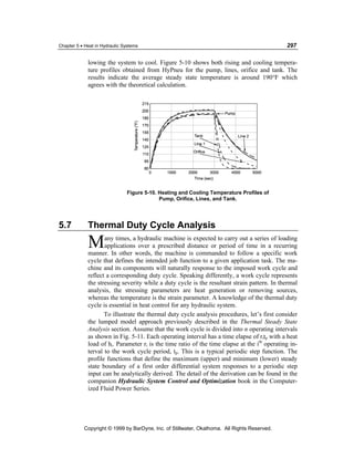
lowing the system to cool. Figure 5-10 shows both rising and cooling tempera-
ture profiles obtained from HyPneu for the pump, lines, orifice and tank. The
results indicate the average steady state temperature is around 190°F which
agrees with the theoretical calculation.
Figure 5-10. Heating and Cooling Temperature Profiles of
Pump, Orifice, Lines, and Tank.
5.7 Thermal Duty Cycle Analysis
M any times, a hydraulic machine is expected to carry out a series of loading
applications over a prescribed distance or period of time in a recurring
manner. In other words, the machine is commanded to follow a specific work
cycle that defines the intended job function to a given application task. The ma-
chine and its components will naturally response to the imposed work cycle and
reflect a corresponding duty cycle. Speaking differently, a work cycle represents
the stressing severity while a duty cycle is the resultant strain pattern. In thermal
analysis, the stressing parameters are heat generation or removing sources,
whereas the temperature is the strain parameter. A knowledge of the thermal duty
cycle is essential in heat control for any hydraulic system.
To illustrate the thermal duty cycle analysis procedures, let’s first consider
the lumped model approach previously described in the Thermal Steady State
Analysis section. Assume that the work cycle is divided into n operating intervals
as shown in Fig. 5-11. Each operating interval has a time elapse of ritp with a heat
load of hi. Parameter ri is the time ratio of the time elapse at the ith operating in-
terval to the work cycle period, tp. This is a typical periodic step function. The
profile functions that define the maximum (upper) and minimum (lower) steady
state boundary of a first order differential system responses to a periodic step
input can be analytically derived. The detail of the derivation can be found in the
companion Hydraulic System Control and Optimization book in the Computer-
ized Fluid Power Series.
Copyright © 1999 by BarDyne, Inc. of Stillwater, Okalhoma. All Rights Reserved.

2. 298 Hydraulic System Design for Service Assurance
Figure 5-11. Periodic Step Function Work Cycle.
However, without getting involved with cumbersome analytical proce-
dures, we can obtain a duty cycle (output) from a given work cycle (input) as
depicted in Fig. 5-12 by the following reasoning. Consider a first order system
with a time constant τ and assume that at time t = 0 both input and output are
null. Right after this point, namely at t = 0+,the input jumps to a new amplitude
U1. Dynamically the output follows an exponential decay curve with the time
constant τ to “catch” the input. At t = t2, the input jumps to the other new ampli-
tude U2. At this moment, the output will immediately change its direction toward
the new equilibrium value even the output has not reach the first equilibrium
value. Note that, at time t2, the output takes the last value before input changed as
the initial point and continues to chase the new equilibrium value exponentially.
This “jump-and-chase” occurs whenever the input changes. Accordingly, the
duty cycle travels between the upper and lower boundaries.
Figure 5-12. Response to a Step-Input Function.
Copyright © 1999 by BarDyne, Inc. of Stillwater, Okalhoma. All Rights Reserved.

3. Chapter 5 • Heat in Hydraulic Systems 299
It is much easier to investigate the duty cycle using computer approach.
Figure 5-13 shows a hydraulic circuit has a 10 gpm pump driving a variable load.
The load is 70% on the low value (around 278 psi), and 30% on the high value
(around 1100) during one work cycle. The equivalent heat loads to the system are
4126 Btu⋅hr-1 for 70% time and 16330 Btu⋅hr-1 for 30%, respectively. Figure 5-14
shows the corresponding oil temperature duty cycle at pump outlet from HyPneu
simulation. It clearly shows that, as expected, the oil temperature travels between
an envelope confined by the upper and lower boundaries.
Figure 5-13. HyPneu Circuit for Thermal Duty Cycle Analysis.
2 00
1 80
Temperature (°F)
1 60
1 40
1 20
1 00
80
0 5 00 1 00 0 1 50 0 2 00 0
T im e (s ec )
Figure 5-14. HyPneu Simulation Results for Thermal Duty Cycle Analysis.
Copyright © 1999 by BarDyne, Inc. of Stillwater, Okalhoma. All Rights Reserved.