For the case of conduction of semi-infinite metal rod in natural convection, we postulate that the temperature profile which satisfies the boundary conditions and the initial condition is the exponential temperature profile. We go ahead and solve the heat equation using this temperature profile and the integral approach and the solution got is used to explain what is observed in the transient and steady state. We notice that the prediction made by the theory is not exactly what is observed with an intercept term which comes in. To account for this intercept, we postulate that there’s convection at the hot end. This accounts for the observed intercept. This analysis can be extended to metal rods of finite length with given boundary conditions and different geometries.

1. Wasswa Derrick 3/4/24 Physics and Mathematics

2. 1

3. 2
TABLE OF CONTENTS
WHAT DO WE OBSERVE EXPERIMENTALLY WHEN HEATING A CYLINDRICAL
METAL ROD AT ONE END WITH WAX PARTICLES ALONG ITS SURFACE AREA? ..3
HOW DO WE DEAL WITH NATURAL CONVECTION AT THE SURFACE AREA OF A
SEMI-INFINITE METAL ROD FOR FIXED WALL TEMPERATURE...................................5
SO HOW DO WE PRODUCE THE SEMI-INFINITE OBSERVED ROD SOLUTION?.15

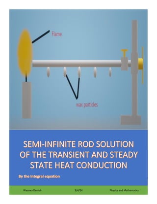
4. 3
WHAT DO WE OBSERVE EXPERIMENTALLY WHEN
HEATING A CYLINDRICAL METAL ROD AT ONE END
WITH WAX PARTICLES ALONG ITS SURFACE AREA?
The situation we are talking about looks as below:
First of all, let us call the distance 𝑥 to be the distance of the wax particle from the hot
end and 𝑡 to be the time taken for the wax to melt since the introduction of the flame
at the hot end.
For a semi-infinite rod(𝑙 = ∞), it is observed that a graph of 𝑥 against time 𝑡 is a curve
as shown below for an aluminium rod of radius 2mm:
A semi-infinite cylindrical rod means that the length of the metal rod extends to
infinity but the radius is finite.
The graph below is for an aluminium rod of length 75cm and radius 2mm and it can
be treated as a semi-infinite metal rod.

5. 4
0
0.05
0.1
0.15
0.2
0.25
0.3
0 100 200 300 400 500
x(metres)
t(seconds)
A Graph of x against time t

6. 5
HOW DO WE DEAL WITH NATURAL CONVECTION AT
THE SURFACE AREA OF A SEMI-INFINITE METAL ROD
FOR FIXED WALL TEMPERATURE
A semi-infinite cylindrical rod means that the length of the metal rod extends to
infinity but the radius of the metal rod is finite. The governing heat equation is:
𝛼
𝜕2
𝑇
𝜕𝑥2
−
ℎ𝑃
𝐴𝜌𝐶
(𝑇 − 𝑇∞) =
𝜕𝑇
𝜕𝑡
We shall use the integral transform approach to solve the heat equation above.
The boundary and initial conditions are
𝑻 = 𝑻𝒔 𝒂𝒕 𝒙 = 𝟎 𝒇𝒐𝒓 𝒂𝒍𝒍 𝒕
𝑻 = 𝑻∞ 𝒂𝒕 𝒙 = ∞
𝑻 = 𝑻∞ 𝒂𝒕 𝒕 = 𝟎
Where: 𝑻∞ = 𝒓𝒐𝒐𝒎 𝒕𝒆𝒎𝒑𝒆𝒓𝒂𝒕𝒖𝒓𝒆
First, we assume a temperature profile that satisfies the boundary conditions as:
𝑇 − 𝑇∞
𝑇𝑠 − 𝑇∞
= 𝑒
−𝑥
𝛿
where 𝛿 is to be determined and is a function of time t and not x.
for the initial condition, we assume 𝛿 = 0 at 𝑡 = 0 seconds so that the initial
condition is satisfied i.e.,
Since at 𝑡 = 0, 𝛿 = 0 we get
𝑇 − 𝑇∞
𝑇𝑠 − 𝑇∞
= 𝑒
−𝑥
0 = 𝑒−∞
= 0
Hence
𝑇 = 𝑇∞
Which is the initial condition.
The governing partial differential equation is:
𝛼
𝜕2
𝑇
𝜕𝑥2
−
ℎ𝑃
𝐴𝜌𝐶
(𝑇 − 𝑇∞) =
𝜕𝑇
𝜕𝑡

7. 6
Let us change transform the heat equation into an integral equation as below:
𝛼 ∫ (
𝜕2
𝑇
𝜕𝑥2
) 𝑑𝑥
𝑙
0
−
ℎ𝑃
𝐴𝜌𝐶
∫ (𝑇 − 𝑇∞)𝑑𝑥
𝑙
0
=
𝜕
𝜕𝑡
∫ (𝑇)𝑑𝑥
𝑙
0
… … . . 𝑏)
𝜕2
𝑇
𝜕𝑥2
=
(𝑇𝑠 − 𝑇∞)
𝛿2
𝑒
−𝑥
𝛿
∫ (
𝜕2
𝑇
𝜕𝑥2
) 𝑑𝑥
𝑙
0
=
−(𝑇𝑠 − 𝑇∞)
𝛿
(𝑒
−𝑙
𝛿 − 1)
But for a semi-infinite cylindrical rod, 𝑙 = ∞, upon substitution, we get
∫ (
𝜕2
𝑇
𝜕𝑥2
) 𝑑𝑥
𝑙
0
=
(𝑇𝑠 − 𝑇∞)
𝛿
∫ (𝑇 − 𝑇∞)𝑑𝑥
𝑙
0
= −𝛿(𝑇𝑠 − 𝑇∞)(𝑒
−𝑙
𝛿 − 1)
But 𝑙 = ∞, upon substitution, we get
∫ (𝑇 − 𝑇∞)𝑑𝑥
𝑙
0
= 𝛿(𝑇𝑠 − 𝑇∞)
𝑇 = (𝑇𝑠 − 𝑇∞)𝑒
−𝑥
𝛿 + 𝑇∞
∫ (𝑇)𝑑𝑥
𝑙
0
= −𝛿(𝑇𝑠 − 𝑇∞)(𝑒
−𝑙
𝛿 − 1) + 𝑇∞𝑙
Substitute 𝑙 = ∞ and get
𝜕
𝜕𝑡
∫ (𝑇)𝑑𝑥
𝑙
0
=
𝑑𝛿
𝑑𝑡
(𝑇𝑠 − 𝑇∞) +
𝜕
𝜕𝑡
(𝑇∞𝑙)
Since 𝑇∞ 𝑎𝑛𝑑 𝑙 are constants
𝜕
𝜕𝑡
(𝑇∞𝑙) = 0
𝜕
𝜕𝑡
∫ (𝑇)𝑑𝑥
𝑙
0
=
𝑑𝛿
𝑑𝑡
(𝑇𝑠 − 𝑇∞)
Substituting the above expressions in equation b) above, we get

8. 7
𝛼 −
ℎ𝑃
𝐴𝜌𝐶
𝛿2
= 𝛿
𝑑𝛿
𝑑𝑡
We solve the equation above with initial condition
𝛿 = 0 𝑎𝑡 𝑡 = 0
And get
𝛿 = √
𝛼𝐴𝜌𝐶
ℎ𝑃
(1 − 𝑒
−2ℎ𝑃
𝐴𝜌𝐶
𝑡
)
𝛿 = √
𝐾𝐴
ℎ𝑃
(1 − 𝑒
−2ℎ𝑃
𝐴𝜌𝐶
𝑡
)
Substituting for 𝛿 in the temperature profile, we get
𝑻 − 𝑻∞
𝑻𝒔 − 𝑻∞
= 𝒆
−𝒙
√
𝑲𝑨
𝒉𝑷
(𝟏−𝒆
−𝟐𝒉𝑷
𝑨𝝆𝑪
𝒕
)
From the equation above, we notice that the initial condition is satisfied i.e.,
𝑻 = 𝑻∞ 𝒂𝒕 𝒕 = 𝟎
The equation above predicts the transient state and in steady state (𝑡 = ∞) it
reduces to
𝑻 − 𝑻∞
𝑻𝒔 − 𝑻∞
= 𝒆
−√(
𝒉𝑷
𝑲𝑨
)𝒙
What are the predictions of the transient state?
For transient state the governing solution is:
𝑇 − 𝑇∞
𝑇𝑠 − 𝑇∞
= 𝑒
−𝑥
√
𝐾𝐴
ℎ𝑃
(1−𝑒
−2ℎ𝑃
𝐴𝜌𝐶
𝑡
)

9. 8
Let us make 𝑥 the subject of the equation of transient state and get:
𝑥 = [ln (
𝑇𝑠 − 𝑇∞
𝑇 − 𝑇∞
)] × √
𝐾𝐴
ℎ𝑃
(1 − 𝑒
−2ℎ𝑃
𝐴𝜌𝐶
𝑡
)
Knowing the thermo-diffusivity, we can measure:
𝑇𝑠1 − 𝑇∞
𝑇 − 𝑇∞
To measure the value of h, we use trial and error method in Microsoft excel and
choosing (
2ℎ𝑃
𝐴𝜌𝐶
= 0.005) , plotting a graph of 𝑥 against √(1 − 𝑒−0.005𝑡) for a semi-
infinite aluminium metal rod of radius 2mm gave a straight-line graph with an
intercept as shown below for all times contrary to the equation above i.e.,
𝑥 = −𝑐 + [ln(
𝑇𝑠 − 𝑇∞
𝑇 − 𝑇∞
)] × √
𝐾𝐴
ℎ𝑃
(1 − 𝑒
−2ℎ𝑃
𝐴𝜌𝐶
𝑡
)
Let:
𝑌 = √(1 − 𝑒−0.005𝑡) = √(1 − 𝑒
−2ℎ𝑃
𝐴𝜌𝐶
𝑡
)
𝒙 = −𝒄 + [𝐥𝐧 (
𝑻𝒔 − 𝑻∞
𝑻 − 𝑻∞
)(√
𝑲𝑨
𝒉𝑷
)] × 𝒀

10. 9
Varying the radius of the aluminium metal rod to 𝑟 = 1𝑚𝑚 the graph looked as
below:
From the graph above, it is observed that the intercept c is directly
proportional to radius squared.
i.e.
𝒄 = 𝟏𝟑𝟗𝟎𝟎𝒓𝟐
The heat transfer coefficient is calculated from
y = 1.515x - 0.0528
R² = 0.9967
0
0.05
0.1
0.15
0.2
0.25
0.3
0 0.05 0.1 0.15 0.2
X
Y
A Graph of X against Y for radius 2mm semi-
infinite aluminium rod
Series1
Linear (Series1)
y = 1.3556x - 0.0139
R² = 0.987
0
0.02
0.04
0.06
0.08
0.1
0.12
0.14
0.16
0.18
0 0.05 0.1 0.15
X
Y
A Graph of X against Y for radius 1mm semi-
infinite aluminium rod
Series1
Linear (Series1)

11. 10
𝑌 = √(1 − 𝑒−0.005𝑡) = √(1 − 𝑒
−2ℎ𝑃
𝐴𝜌𝐶
𝑡
)
2ℎ𝑃
𝐴𝜌𝐶
= 0.005
h for aluminium was found to be
ℎ =
6.075𝑊
𝑚2𝐾
Using the graph and the equation below:
𝑥 = [ln (
𝑇𝑓 − 𝑇∞
𝑇 − 𝑇∞
)] × √
𝐾𝐴
ℎ𝑃
(1 − 𝑒
−2ℎ𝑃
𝐴𝜌𝐶
𝑡
) − 𝛽𝑟
From the gradient of the graph of x against √(1 − 𝑒
−2ℎ𝑃
𝐴𝜌𝐶
𝑡
)above the ratio (
𝑇𝑓−𝑇∞
𝑇−𝑇∞
)
was measured and was found to be:
(
𝑻 − 𝑻∞
𝑻𝒇 − 𝑻∞
) ≈ 𝟎. 𝟐𝟏𝟗𝟖𝟏
From the graph above it is deduced that 𝑇𝑓 is a constant temperature
independent of time.
To account for the intercept in the graph above for a semi-infinite rod, we have
to postulate that there’s convection at the hot end of the metal rod as below
i.e.,

12. 11
−𝒌
𝝏𝑻
𝝏𝒙
|𝒙=𝟎 = 𝒉𝟎(𝑻𝒇 − 𝑻𝒔)
Recall:
𝑇 − 𝑇∞
𝑇𝑠 − 𝑇∞
= 𝑒
−𝑥
𝛿
𝜕𝑇
𝜕𝑥
=
−(𝑇𝑠 − 𝑇∞)
𝛿
𝑒
−𝑥
𝛿
𝜕𝑇
𝜕𝑥
|𝑥=0 =
−(𝑇𝑠 − 𝑇∞)
𝛿
Upon substitution, we get:
𝑘
(𝑇𝑠 − 𝑇∞)
𝛿
= ℎ0(𝑇𝑓 − 𝑇𝑠)
(𝑇𝑠 − 𝑇∞) =
ℎ0𝛿
𝑘
(𝑇𝑓 − 𝑇𝑠)
𝑇𝑠 (1 +
ℎ0𝛿
𝑘
) = (
ℎ0𝛿
𝑘
) 𝑇𝑓 + 𝑇∞
𝑇𝑠 =
(
ℎ0𝛿
𝑘
) 𝑇𝑓 + 𝑇∞
(1 +
ℎ0𝛿
𝑘
)
Subtracting 𝑇∞ from both sides, we get:

13. 12
𝑇𝑠 − 𝑇∞ =
(
ℎ0𝛿
𝑘
) 𝑇𝑓 + 𝑇∞
(1 +
ℎ0𝛿
𝑘
)
− 𝑇∞
We finally get:
𝑇𝑠 − 𝑇∞
𝑇𝑓 − 𝑇∞
=
ℎ0𝛿
𝑘
1 +
ℎ0𝛿
𝑘
Upon simplifying, we get:
𝑇𝑠 − 𝑇∞
𝑇𝑓 − 𝑇∞
=
𝛿
𝛿 +
𝑘
ℎ0
To explain the nature of ℎ0 we postulate that the candle dissipates power
independent of area. i.e.,
𝑑𝑚
𝑑𝑡
𝐻𝐶 = 𝛾ℎ0𝐴(𝑇𝑓 − 𝑇𝑠)
Where:
𝛾 = 𝑝𝑟𝑜𝑝𝑜𝑟𝑡𝑖𝑜𝑛𝑎𝑙𝑖𝑡𝑦 𝑐𝑜𝑛𝑠𝑡𝑎𝑛𝑡 𝑎𝑛𝑑 𝑐𝑎𝑛 𝑏𝑒 𝑡𝑎𝑘𝑒𝑛 𝑡𝑜 𝑏𝑒 𝑒𝑞𝑢𝑎𝑙 𝑡𝑜 1
And get
𝒅𝒎
𝒅𝒕
𝑯𝑪 = 𝒉𝟎𝑨(𝑻𝒇 − 𝑻𝒔)
Where:
𝐻𝐶 = 𝑒𝑛𝑡ℎ𝑎𝑙𝑝𝑦 𝑜𝑓 𝑐𝑜𝑚𝑏𝑢𝑠𝑡𝑖𝑜𝑛
From experiment:
𝑑𝑚
𝑑𝑡
= 𝑐𝑜𝑛𝑠𝑡𝑎𝑛𝑡
To explain the heat conduction phenomenon, we postulate that
𝐻𝐶 = 𝐶𝑜(𝑇𝑓 − 𝑇𝑠)
Where:

14. 13
𝐶𝑜 = 𝑠𝑝𝑒𝑐𝑖𝑓𝑖𝑐 ℎ𝑒𝑎𝑡 𝑐𝑎𝑝𝑎𝑐𝑖𝑡𝑦
Upon substitution, we have:
𝑑𝑚
𝑑𝑡
𝐶𝑜(𝑇𝑓 − 𝑇𝑠) = ℎ0𝐴(𝑇𝑓 − 𝑇𝑠)
Upon simplifying, we get:
𝒉𝟎 =
𝒅𝒎
𝒅𝒕
×
𝑪𝒐
𝑨
Using the above result, we get
𝑘
ℎ0
=
𝑘𝐴
𝑑𝑚
𝑑𝑡
𝐶𝑜
Upon substitution, we get:
𝑇𝑠 − 𝑇∞
𝑇𝑓 − 𝑇∞
=
𝛿
𝛿 +
𝑘
ℎ0
𝑇𝑠 − 𝑇∞
𝑇𝑓 − 𝑇∞
=
𝛿
𝛿 +
𝑘𝐴
𝑑𝑚
𝑑𝑡
𝐶𝑜
OR
𝑇𝑠 − 𝑇∞
𝑇𝑓 − 𝑇∞
=
𝛿
𝛿 +
𝑘𝜋
𝑑𝑚
𝑑𝑡
𝐶𝑜
𝑟2
Comparing with:
𝑻𝒔 − 𝑻∞
𝑻𝒇 − 𝑻∞
=
𝜹
𝜹 + 𝜷𝒓𝟐
Where:
𝛽 =
𝑘𝜋
𝑑𝑚
𝑑𝑡
𝐶𝑜

15. 14
We notice that 𝛽 is directly proportional to the thermal conductivity k.
The above expression shows that the temperature at 𝑥 = 0 varies with time also
and is not fixed until steady state is achieved
𝒌
𝒉𝟎
= 𝜷𝒓𝟐
And we finally get:
𝑇𝑠 − 𝑇∞
𝑇𝑓 − 𝑇∞
=
𝛿
𝛿 + 𝛽𝑟2
For a semi-infinite rod,
𝑻 − 𝑻∞
𝑻𝒔 − 𝑻∞
= 𝒆−
𝒙
𝜹
Substituting the expression of (𝑇𝑠 − 𝑇∞) we get:
𝑻 − 𝑻∞
𝑻𝒇 − 𝑻∞
= (
𝜹
𝜹 + 𝜷𝒓𝟐
)𝒆−
𝒙
𝜹
As the general solution.

16. 15
SO HOW DO WE PRODUCE THE SEMI-INFINITE OBSERVED ROD
SOLUTION?
As got before:
𝑇𝑠 − 𝑇∞
𝑇𝑓 − 𝑇∞
= (
𝛿
𝛿 + 𝛽𝑟2
)
From
(
𝑻 − 𝑻∞
𝑻𝒔 − 𝑻∞
) = 𝒆−
𝒙
𝜹
Substituting the expression of (𝑇𝑠 − 𝑇∞) we get:
𝑻 − 𝑻∞
𝑻𝒇 − 𝑻∞
= (
𝜹
𝜹 + 𝜷𝒓𝟐
)𝒆−
𝒙
𝜹
Continuing with
𝑻 − 𝑻∞
𝑻𝒔 − 𝑻∞
= 𝒆−
𝒙
𝜹
Let us make 𝑥 the subject of the formula:
𝑥 = [ln(
𝑇𝑠 − 𝑇∞
𝑇 − 𝑇∞
)] × 𝛿
Where:
𝛿 = √2𝛼𝑡
For small time.
Or generally
𝛿 = √
𝐾𝐴
ℎ𝑃
(1 − 𝑒
−2ℎ𝑃
𝐴𝜌𝐶
𝑡
)
But we know from the above that:
(𝑇𝑠 − 𝑇∞) = (𝑇𝑓 − 𝑇∞)(
𝛿
𝛿 + 𝛽𝑟2
)
𝑥 = [ln(𝑇𝑠 − 𝑇∞) − ln(𝑇 − 𝑇∞)] × 𝛿
𝑙𝑛(𝑇𝑠 − 𝑇∞) = 𝑙𝑛(𝑇𝑓 − 𝑇∞) + 𝑙𝑛(
𝛿
𝛿 + 𝛽𝑟2
)

17. 16
Upon substitution of 𝑙𝑛(𝑇𝑠 − 𝑇∞) in the equation of 𝑥 above, we get
𝑥 = [𝑙𝑛(𝑇𝑓 − 𝑇∞) + 𝑙𝑛(
𝛿
𝛿 + 𝛽𝑟2
) −ln(𝑇 − 𝑇∞)] × 𝛿
We get
𝒙 = 𝜹[𝒍𝒏 (
𝑻𝒇 − 𝑻∞
𝑻 − 𝑻∞
) + 𝒍𝒏(
𝜹
𝜹 + 𝜷𝒓𝟐
)]
Let us manipulate the equation above and get:
𝒙 = 𝜹𝒍𝒏 (
𝑻𝒇 − 𝑻∞
𝑻 − 𝑻∞
) + 𝜹𝒍𝒏(
𝜹
𝜹 + 𝜷𝒓𝟐
)
Factorizing out 𝛿 in the denominator we get:
𝑥 = 𝛿𝑙𝑛 (
𝑇𝑓 − 𝑇∞
𝑇 − 𝑇∞
) + 𝛿𝑙𝑛[
𝛿
𝛿
(
1
1 +
𝛽𝑟2
𝛿
)]
𝑥 = 𝛿𝑙𝑛 (
𝑇𝑓 − 𝑇∞
𝑇 − 𝑇∞
) + 𝛿𝑙𝑛[(1 +
𝛽𝑟2
𝛿
)−1
]
Since
𝛽𝑟2
𝛿
≪ 1 𝑓𝑜𝑟 𝑡
We can use the binomial first order approximation
(1 + 𝑥)𝑛
≈ 1 + 𝑛𝑥 𝑓𝑜𝑟 𝑥 ≪ 1
(1 +
𝛽𝑟2
𝛿
)−1
= 1 −
𝛽𝑟2
𝛿
𝑓𝑜𝑟
𝛽𝑟2
𝛿
≪ 1
And we get:
𝑥 = 𝛿𝑙𝑛 (
𝑇𝑓 − 𝑇∞
𝑇 − 𝑇∞
) + 𝛿𝑙𝑛[(1 −
𝛽𝑟2
𝛿
)]
Again, we can expand the natural log as below:
ln(1 − 𝑥) ≈ −𝑥 𝑓𝑜𝑟 𝑥 ≪ 1
𝑙𝑛 [(1 −
𝛽𝑟2
𝛿
)] = −
𝛽𝑟2
𝛿
𝑓𝑜𝑟
𝛽𝑟2
𝛿
≪ 1

18. 17
Upon substitution we finally get
𝒙 = 𝜹𝒍𝒏 (
𝑻𝒇 − 𝑻∞
𝑻 − 𝑻∞
) − 𝜷𝒓𝟐
Which is what we got before.
𝒙 = 𝜹𝒍𝒏 (
𝑻𝒇 − 𝑻∞
𝑻 − 𝑻∞
) − 𝜷𝒓𝟐
Where:
𝛽 =
𝑘𝜋
𝑑𝑚
𝑑𝑡
𝐶𝑜
We notice that the intercept above is proportional to the square of the radius as
demonstrated from experiment.
Looking at the general solution:
𝒙 = 𝜹𝒍𝒏 (
𝑻𝒇 − 𝑻∞
𝑻 − 𝑻∞
) + 𝜹𝒍𝒏(
𝜹
𝜹 + 𝜷𝒓𝟐
)
Plotting a graph of 𝒙 against 𝜹[𝒍𝒏 (
𝑻𝒇−𝑻∞
𝑻−𝑻∞
) + 𝒍𝒏(
𝜹
𝜹+𝜷𝒓𝟐
)] was found to give a
straight-line graph through the origin as stated by the equation above.
Let us call 𝒑 = 𝜹[𝒍𝒏 (
𝑻𝒇−𝑻∞
𝑻−𝑻∞
) + 𝒍𝒏(
𝜹
𝜹+𝜷𝒓𝟐
)]
Where:
𝜷𝒓𝟐
= 𝟎. 𝟎𝟓𝟐𝟖 for an aluminium rod of radius 2mm and 𝐾 = 238
𝑊
𝑚𝐾
, ℎ = 6
𝑊
𝑚2𝐾
𝜌 =
2700
𝑘𝑔
𝑚3, 𝐶 = 900
𝐽
𝑘𝑔𝐾
and
𝑇−𝑇∞
𝑇𝑓−𝑇∞
= 0.21981
And
𝛿 = √
𝐾𝐴
ℎ𝑃
(1 − 𝑒
−2ℎ𝑃
𝐴𝜌𝐶
𝑡
)
Then a graph of x against p is a straight-line graph through the origin for a
semi-infinite rod as shown below for a semi-infinite aluminium rod of radius
2mm

19. 18
Calling the solution below the approximated solution:
𝒙 = 𝜹𝒍𝒏 (
𝑻𝒇 − 𝑻∞
𝑻 − 𝑻∞
) − 𝜷𝒓𝟐
Or
𝑥 = [ln (
𝑇𝑓 − 𝑇∞
𝑇 − 𝑇∞
)] × √
𝐾𝐴
ℎ𝑃
(1 − 𝑒
−2ℎ𝑃
𝐴𝜌𝐶
𝑡
) − 𝛽𝑟2
What are the lessons we have learnt?
 We have learnt that in the approximated solution, we can measure off h
in the transient state.
 We have learnt that knowing the thermo-conductivity and other physical
parameters of the metal rod, in the approximated solution, we can
measure off the ratio
𝑻−𝑻∞
𝑻𝒇−𝑻∞
 The intercept in the approximated solution can help us learn how its
nature varies with the radius of the rod. We can use the intercept to
measure the value of 𝜷.
y = 1.0768x
0
0.05
0.1
0.15
0.2
0.25
0.3
0 0.05 0.1 0.15 0.2 0.25
x
p
A Graph of x against p

20. 19
The general solution is given by:
𝒙 = 𝜹𝒍𝒏 (
𝑻𝒇 − 𝑻∞
𝑻 − 𝑻∞
) + 𝜹𝒍𝒏(
𝜹
𝜹 + 𝜷𝒓𝟐
)
You notice that the initial condition is still satisfied.
From the general solution, we get:
𝑻 − 𝑻∞
𝑻𝒇 − 𝑻∞
= (
𝜹
𝜹 + 𝜷𝒓𝟐
)𝒆
−
𝒙
𝜹
For the initial condition; At 𝑡 = 0, you get
𝑻 − 𝑻∞
𝑻𝒇 − 𝑻∞
= 𝟎 × 𝒆
−𝒙
𝟎 = 𝟎
Hence
𝑻 = 𝑻∞
Considering the approximated equation below:
𝒙 = [𝐥𝐧 (
𝑻𝒇 − 𝑻∞
𝑻 − 𝑻∞
)] × √𝟐𝜶𝒕 − 𝜷𝒓𝟐
What that equation says is that when you stick wax particles on a long metal
rod (𝑙 = ∞) at distances x from the hot end of the rod and note the time t it
takes the wax particles to melt, then a graph of 𝑥 against √𝑡 is a straight-line
graph with an intercept as stated by the equation above when the times are
small. The equation is true because that is what is observed experimentally.
Looking at the approximate solution for a semi-infinite metal rod:
𝑥 = −𝛽𝑟2
+ [ln(
𝑇𝑓 − 𝑇∞
𝑇 − 𝑇∞
)] × √
𝐾𝐴
ℎ𝑃
(1 − 𝑒
−2ℎ𝑃
𝐴𝜌𝐶
𝑡
)
Let:
𝑌 = √(1 − 𝑒−0.005𝑡)
A graph of x against Y looked as below:

21. 20
Since the graph above is a straight-line graph, it shows that 𝑇𝑓 IS NOT a
function of time as stated by the equation above of 𝑥 against Y.
Another point to note is that from experiment 𝑇𝑓 was found to be independent
of radius of the metal rod.
For aluminium
𝐾 = 238
𝑊
𝑚𝐾
, ℎ = 6
𝑊
𝑚2𝐾
Another way to measure 𝑇𝑠1 is to consider the steady state equation and plot
the graph of
𝑇 − 𝑇∞
𝑇𝑓 − 𝑇∞
= (
𝛿
𝛿 + 𝛽𝑟2
)𝑒
−√(
ℎ𝑃
𝐾𝐴)𝑥
𝐥𝐧(𝑻 − 𝑻∞) = 𝒍𝒏(𝑻𝒇 − 𝑻∞) + 𝒍𝒏(
𝜹
𝜹 + 𝜷𝒓𝟐
) − √(
𝒉𝑷
𝑲𝑨
)𝒙
And
𝛿 = √
𝐾𝐴
ℎ𝑃
Upon substitution
y = 1.515x - 0.0528
R² = 0.9967
0
0.05
0.1
0.15
0.2
0.25
0.3
0 0.05 0.1 0.15 0.2
X
Y
A Graph of X against Y
Series1
Linear (Series1)

22. 21
𝐥𝐧(𝑻 − 𝑻∞) = 𝒍𝒏(𝑻𝒇 − 𝑻∞) + 𝒍𝒏(
√𝑲𝑨
𝒉𝑷
√𝑲𝑨
𝒉𝑷
+ 𝜷𝒓𝟐
) − √(
𝒉𝑷
𝑲𝑨
)𝒙
A graph of ln(𝑇 − 𝑇∞) against x gives an intercept [𝒍𝒏(𝑻𝒇 − 𝑻∞) + 𝒍𝒏(
√
𝑲𝑨
𝒉𝑷
√
𝑲𝑨
𝒉𝑷
+𝜷𝒓𝟐
)] from
which 𝑇𝑓 can be measured.
Also knowing the thermo-conductivity, from the gradient of the above graph the
heat transfer coefficient can be measured off.
From experiment, using an aluminium rod of radius 2mm and using a
thermoconductivity value of 𝟐𝟑𝟖 𝑾
𝒎𝑲
⁄ , The heat transfer coefficient h of
aluminium was found to be 𝟔 𝑾
𝒎𝟐𝑲
⁄ .
Therefore, for a semi-infinite rod, the equation obeyed for small times is:
𝒙 = [𝐥𝐧 (
𝑻𝒇 − 𝑻∞
𝑻 − 𝑻∞
)] × √𝟐𝜶𝒕 − 𝜷𝒓𝟐
Looking at the steady state solution below:
𝑇 − 𝑇∞
𝑇𝑓 − 𝑇∞
= (
𝛿
𝛿 + 𝛽𝑟2
)𝑒
−√(
ℎ𝑃
𝐾𝐴
)𝑥
OR
𝑻 − 𝑻∞
𝑻𝒇 − 𝑻∞
= (
√𝑲𝑨
𝒉𝑷
√𝑲𝑨
𝒉𝑷
+ 𝜷𝒓𝟐
)𝒆
−√(
𝒉𝑷
𝑲𝑨
)𝒙
In most cases
√
𝑲𝑨
𝒉𝑷
≫ 𝜷𝒓𝟐
So, we observe:

23. 22
𝑻 − 𝑻∞
𝑻𝒇 − 𝑻∞
= 𝒆
−√(
𝒉𝑷
𝑲𝑨
)𝒙
Which is the usual solution we know.
From experiment, using a flame and candle wax on the aluminium rod, the
ratio below was found to be
(
𝑻 − 𝑻∞
𝑻𝒇 − 𝑻∞
) ≈ 𝟎. 𝟐𝟏𝟗𝟖𝟏