Here are the key claims, findings, and conclusions from the text: Claims: - Transient state heat transfer in a cylindrical metal rod with one end heated can be modeled mathematically. - The temperature profile along the rod depends on whether the rod is semi-infinite or finite. - There is convection at the heated end of the rod as investigated experimentally in addition to conduction along the rod. Findings: - For a semi-infinite rod, the temperature profile decays exponentially with distance from the heated end. - For a finite rod with no flux at the far end, the temperature profile involves hyperbolic cosine functions. - For a finite rod with convection at the far end, the temperature profile also depends on hyperbolic sine functions. - The models match experimental measurements of melting wax particles along aluminum rods. We deduce from experiment that there’s convection at the hot end and that the heat transfer coefficient at the far end varies with length of the metal rod. Conclusions: - The integral transform approach allows deriving temperature profiles satisfying boundary conditions. - There is convection at the hot end, and the heat transfer coefficient at the far end varies with length L as investigated experimentally. - The simple models provide good agreement with experimental temperature profiles in aluminum rods. In summary, the text presents mathematical models of heat transfer in metal rods that agree with experiments and provide insight into the temperature profiles by considering different boundary conditions. The key findings relate to the functional forms of the temperature profiles in semi-infinite versus finite rods.

1. Wasswa Derrick 3/4/24 Heat Conduction

3. TABLE OF CONTENTS
PREFACE ............................................................................................................................................3
WHAT DO WE OBSERVE EXPERIMENTALLY WHEN HEATING A CYLINDRICAL
METAL ROD AT ONE END WITH WAX PARTICLES ALONG ITS SURFACE AREA? ..4
HOW DO WE DEAL WITH NATURAL CONVECTION AT THE SURFACE AREA OF A
SEMI-INFINITE METAL ROD FOR FIXED WALL TEMPERATURE...................................6
SO HOW DO WE PRODUCE THE SEMI-INFINITE OBSERVED ROD SOLUTION?.16
HOW DOES HEAT FLOW MANIFEST ITSELF FOR FINITE METAL RODS? ...............26
CASE 1: CONVECTION AT THE END OF A FINITE METAL ROD...............................26
HOW DO WE INVESTIGATE THE NATURE OF 𝒉𝑳 EASILY?.....................................31
DERIVATION OF THE GENERAL EXPRESSION FOR HEAT TRANSFER
COEFFICIENT 𝒉𝑳........................................................................................................................39
CASE 2: ZERO FLUX AT THE END OF THE METAL ROD?..........................................44
HOW DO WE DEAL WITH CYLINDRICAL COORDINATES? .............................................50
HOW DO WE DEAL WITH CYLINDRICAL CO-ORDINATES FOR A SEMI-INFINITE
RADIUS CYLINDER? .....................................................................................................................51
HOW DO WE DEAL WITH NATURAL CONVECTION AT THE SURFACE AREA OF A
SEMI-INFINITE CYLINDER FOR FIXED END TEMPERATURE.......................................54
REFERENCES..................................................................................................................................58

4. PREFACE
In this book we go ahead and investigate the nature of heat conduction in a
metal rod heated at one end while the other end is free. We do this by sticking
wax particles along the surface area of the metal rod at known distances x from
the hot end and then record the time taken for each wax to melt since the
introduction of the flame at the hot end. We first of all look at the case of heat
conduction in a semi-infinite metal rod and solve the heat equation analytically
using the integral transform approach and compare the solution got in the
transient state to experimental observations. We make deductions and
conclusions from both the solution and the experimental values.
We then look at the case of a finite length metal rod heat conduction with
convection at the free end. We use the hyperbolic function solutions known in
literature to interpret experimental data. One fact that we get to learn from the
experimental values is that the heat transfer coefficient ℎ𝐿 at the end of the
metal rod is not a constant but varies with length L as shall be shown later. We
note that in deriving the solution for the convection boundary condition, the
solution derived should reduce to the semi-infinite rod solution as the length
tends to infinity.
We then look at the case of zero flux at the end of a finite metal rod and also
derive the governing equation.
Finally, we use the integral approach to solve the heat equation in cylindrical
co-ordinates for radial heat conduction and use the same techniques we used
before to solve for observed phenomena.

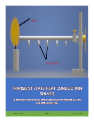
5. WHAT DO WE OBSERVE EXPERIMENTALLY WHEN
HEATING A CYLINDRICAL METAL ROD AT ONE END
WITH WAX PARTICLES ALONG ITS SURFACE AREA?
The situation we are talking about looks as below:
First of all, let us call the distance 𝑥 to be the distance of the wax particle from the hot
end and 𝑡 to be the time taken for the wax to melt since the introduction of the flame
at the hot end.
For a semi-infinite rod(𝑙 = ∞), it is observed that a graph of 𝑥 against time 𝑡 is a curve
as shown below for an aluminium rod of radius 2mm:
A semi-infinite cylindrical rod means that the length of the metal rod extends to
infinity but the radius is finite.
The graph below is for an aluminium rod of length 75cm and radius 2mm and it can
be treated as a semi-infinite metal rod.

6. 0
0.05
0.1
0.15
0.2
0.25
0.3
0 100 200 300 400 500
x(metres)
t(seconds)
A Graph of x against time t

7. HOW DO WE DEAL WITH NATURAL CONVECTION AT
THE SURFACE AREA OF A SEMI-INFINITE METAL ROD
FOR FIXED WALL TEMPERATURE
A semi-infinite cylindrical rod means that the length of the metal rod extends to
infinity but the radius of the metal rod is finite. The governing heat equation is:
𝛼
𝜕2
𝑇
𝜕𝑥2
−
ℎ𝑃
𝐴𝜌𝐶
(𝑇 − 𝑇∞) =
𝜕𝑇
𝜕𝑡
We shall use the integral transform approach to solve the heat equation above.
The boundary and initial conditions are
𝑻 = 𝑻𝒔 𝒂𝒕 𝒙 = 𝟎 𝒇𝒐𝒓 𝒂𝒍𝒍 𝒕
𝑻 = 𝑻∞ 𝒂𝒕 𝒙 = ∞
𝑻 = 𝑻∞ 𝒂𝒕 𝒕 = 𝟎
Where: 𝑻∞ = 𝒓𝒐𝒐𝒎 𝒕𝒆𝒎𝒑𝒆𝒓𝒂𝒕𝒖𝒓𝒆
First, we assume a temperature profile that satisfies the boundary conditions as:
𝑇 − 𝑇∞
𝑇𝑠 − 𝑇∞
= 𝑒
−𝑥
𝛿
where 𝛿 is to be determined and is a function of time t and not x.
for the initial condition, we assume 𝛿 = 0 at 𝑡 = 0 seconds so that the initial
condition is satisfied i.e.,
Since at 𝑡 = 0, 𝛿 = 0 we get
𝑇 − 𝑇∞
𝑇𝑠 − 𝑇∞
= 𝑒
−𝑥
0 = 𝑒−∞
= 0
Hence
𝑇 = 𝑇∞
Which is the initial condition.
The governing partial differential equation is:
𝛼
𝜕2
𝑇
𝜕𝑥2
−
ℎ𝑃
𝐴𝜌𝐶
(𝑇 − 𝑇∞) =
𝜕𝑇
𝜕𝑡

8. Let us change transform the heat equation into an integral equation as below:
𝛼 ∫ (
𝜕2
𝑇
𝜕𝑥2
) 𝑑𝑥
𝑙
0
−
ℎ𝑃
𝐴𝜌𝐶
∫ (𝑇 − 𝑇∞)𝑑𝑥
𝑙
0
=
𝜕
𝜕𝑡
∫ (𝑇)𝑑𝑥
𝑙
0
… … . . 𝑏)
𝜕2
𝑇
𝜕𝑥2
=
(𝑇𝑠 − 𝑇∞)
𝛿2
𝑒
−𝑥
𝛿
∫ (
𝜕2
𝑇
𝜕𝑥2
) 𝑑𝑥
𝑙
0
=
−(𝑇𝑠 − 𝑇∞)
𝛿
(𝑒
−𝑙
𝛿 − 1)
But for a semi-infinite cylindrical rod, 𝑙 = ∞, upon substitution, we get
∫ (
𝜕2
𝑇
𝜕𝑥2
) 𝑑𝑥
𝑙
0
=
(𝑇𝑠 − 𝑇∞)
𝛿
∫ (𝑇 − 𝑇∞)𝑑𝑥
𝑙
0
= −𝛿(𝑇𝑠 − 𝑇∞)(𝑒
−𝑙
𝛿 − 1)
But 𝑙 = ∞, upon substitution, we get
∫ (𝑇 − 𝑇∞)𝑑𝑥
𝑙
0
= 𝛿(𝑇𝑠 − 𝑇∞)
𝑇 = (𝑇𝑠 − 𝑇∞)𝑒
−𝑥
𝛿 + 𝑇∞
∫ (𝑇)𝑑𝑥
𝑙
0
= −𝛿(𝑇𝑠 − 𝑇∞)(𝑒
−𝑙
𝛿 − 1) + 𝑇∞𝑙
Substitute 𝑙 = ∞ and get
𝜕
𝜕𝑡
∫ (𝑇)𝑑𝑥
𝑙
0
=
𝑑𝛿
𝑑𝑡
(𝑇𝑠 − 𝑇∞) +
𝜕
𝜕𝑡
(𝑇∞𝑙)
Since 𝑇∞ 𝑎𝑛𝑑 𝑙 are constants
𝜕
𝜕𝑡
(𝑇∞𝑙) = 0
𝜕
𝜕𝑡
∫ (𝑇)𝑑𝑥
𝑙
0
=
𝑑𝛿
𝑑𝑡
(𝑇𝑠 − 𝑇∞)
Substituting the above expressions in equation b) above, we get

9. 𝛼 −
ℎ𝑃
𝐴𝜌𝐶
𝛿2
= 𝛿
𝑑𝛿
𝑑𝑡
We solve the equation above with initial condition
𝛿 = 0 𝑎𝑡 𝑡 = 0
And get
𝛿 = √
𝛼𝐴𝜌𝐶
ℎ𝑃
(1 − 𝑒
−2ℎ𝑃
𝐴𝜌𝐶
𝑡
)
𝛿 = √
𝐾𝐴
ℎ𝑃
(1 − 𝑒
−2ℎ𝑃
𝐴𝜌𝐶
𝑡
)
Substituting for 𝛿 in the temperature profile, we get
𝑻 − 𝑻∞
𝑻𝒔 − 𝑻∞
= 𝒆
−𝒙
√
𝑲𝑨
𝒉𝑷
(𝟏−𝒆
−𝟐𝒉𝑷
𝑨𝝆𝑪
𝒕
)
From the equation above, we notice that the initial condition is satisfied i.e.,
𝑻 = 𝑻∞ 𝒂𝒕 𝒕 = 𝟎
The equation above predicts the transient state and in steady state (𝑡 = ∞) it
reduces to
𝑻 − 𝑻∞
𝑻𝒔 − 𝑻∞
= 𝒆
−√(
𝒉𝑷
𝑲𝑨
)𝒙
What are the predictions of the transient state?
For transient state the governing solution is:
𝑇 − 𝑇∞
𝑇𝑠 − 𝑇∞
= 𝑒
−𝑥
√
𝐾𝐴
ℎ𝑃
(1−𝑒
−2ℎ𝑃
𝐴𝜌𝐶
𝑡
)

10. Let us make 𝑥 the subject of the equation of transient state and get:
𝑥 = [ln (
𝑇𝑠 − 𝑇∞
𝑇 − 𝑇∞
)] × √
𝐾𝐴
ℎ𝑃
(1 − 𝑒
−2ℎ𝑃
𝐴𝜌𝐶
𝑡
)
To measure the value of h, we use trial and error method in Microsoft excel and
choosing (
2ℎ𝑃
𝐴𝜌𝐶
= 0.005) , plotting a graph of 𝑥 against √(1 − 𝑒−0.005𝑡) for a semi-
infinite aluminium metal rod of radius 2mm gave a straight-line graph with a
negative intercept as shown below for all times contrary to the equation
above i.e.,
𝑥 = −𝑐 + [ln(
𝑇𝑠 − 𝑇∞
𝑇 − 𝑇∞
)] × √
𝐾𝐴
ℎ𝑃
(1 − 𝑒
−2ℎ𝑃
𝐴𝜌𝐶
𝑡
)
Let:
𝑌 = √(1 − 𝑒−0.005𝑡) = √(1 − 𝑒
−2ℎ𝑃
𝐴𝜌𝐶
𝑡
)
𝒙 = −𝒄 + [𝐥𝐧 (
𝑻𝒔 − 𝑻∞
𝑻 − 𝑻∞
)(√
𝑲𝑨
𝒉𝑷
)] × 𝒀

11. Varying the radius of the aluminium metal rod to 𝑟 = 1𝑚𝑚 the graph looked as
below:
From the graph above, it is observed that the intercept c is directly proportional
to radius squared.
i.e.
𝒄 = 𝟏𝟑𝟗𝟎𝟎𝒓𝟐
The heat transfer coefficient is calculated from
y = 1.515x - 0.0528
R² = 0.9967
0
0.05
0.1
0.15
0.2
0.25
0.3
0 0.05 0.1 0.15 0.2
X
Y
A Graph of X against Y for radius 2mm semi-
infinite aluminium rod
Series1
Linear (Series1)
y = 1.3556x - 0.0139
R² = 0.987
0
0.02
0.04
0.06
0.08
0.1
0.12
0.14
0.16
0.18
0 0.05 0.1 0.15
X
Y
A Graph of X against Y for radius 1mm semi-
infinite aluminium rod
Series1
Linear (Series1)

12. 𝑌 = √(1 − 𝑒−0.005𝑡) = √(1 − 𝑒
−2ℎ𝑃
𝐴𝜌𝐶
𝑡
)
2ℎ𝑃
𝐴𝜌𝐶
= 0.005
h for aluminium was found to be
ℎ =
6.075𝑊
𝑚2𝐾
Using the graph and the equation below:
𝑥 = [ln (
𝑇𝑓 − 𝑇∞
𝑇 − 𝑇∞
)] × √
𝐾𝐴
ℎ𝑃
(1 − 𝑒
−2ℎ𝑃
𝐴𝜌𝐶
𝑡
) − 𝛽𝑟2
From the gradient of the graph of x against √(1 − 𝑒
−2ℎ𝑃
𝐴𝜌𝐶
𝑡
)above the ratio (
𝑇𝑓−𝑇∞
𝑇−𝑇∞
)
was measured and was found to be:
(
𝑻 − 𝑻∞
𝑻𝒇 − 𝑻∞
) ≈ 𝟎. 𝟐𝟏𝟗𝟖𝟏
From the graph above it is deduced that 𝑇𝑓 is a constant temperature
independent of time.
To account for the intercept in the graph above for a semi-infinite rod, we have
to postulate that there’s convection at the hot end of the metal rod as below
i.e.,

13. −𝒌
𝝏𝑻
𝝏𝒙
|𝒙=𝟎 = 𝒉𝟎(𝑻𝒇 − 𝑻𝒔)
Recall:
𝑇 − 𝑇∞
𝑇𝑠 − 𝑇∞
= 𝑒
−𝑥
𝛿
𝜕𝑇
𝜕𝑥
=
−(𝑇𝑠 − 𝑇∞)
𝛿
𝑒
−𝑥
𝛿
𝜕𝑇
𝜕𝑥
|𝑥=0 =
−(𝑇𝑠 − 𝑇∞)
𝛿
Upon substitution, we get:
𝑘
(𝑇𝑠 − 𝑇∞)
𝛿
= ℎ0(𝑇𝑓 − 𝑇𝑠)
(𝑇𝑠 − 𝑇∞) =
ℎ0𝛿
𝑘
(𝑇𝑓 − 𝑇𝑠)
𝑇𝑠 (1 +
ℎ0𝛿
𝑘
) = (
ℎ0𝛿
𝑘
) 𝑇𝑓 + 𝑇∞
𝑇𝑠 =
(
ℎ0𝛿
𝑘
) 𝑇𝑓 + 𝑇∞
(1 +
ℎ0𝛿
𝑘
)
Subtracting 𝑇∞ from both sides, we get:

14. 𝑇𝑠 − 𝑇∞ =
(
ℎ0𝛿
𝑘
) 𝑇𝑓 + 𝑇∞
(1 +
ℎ0𝛿
𝑘
)
− 𝑇∞
We finally get:
𝑇𝑠 − 𝑇∞
𝑇𝑓 − 𝑇∞
=
ℎ0𝛿
𝑘
1 +
ℎ0𝛿
𝑘
Upon simplifying, we get:
𝑇𝑠 − 𝑇∞
𝑇𝑓 − 𝑇∞
=
𝛿
𝛿 +
𝑘
ℎ0
To explain the nature of ℎ0 we postulate that the candle dissipates power
independent of area. i.e.,
𝑑𝑚
𝑑𝑡
𝐻𝐶 = 𝛾ℎ0𝐴(𝑇𝑓 − 𝑇𝑠)
Where:
𝛾 = 𝑝𝑟𝑜𝑝𝑜𝑟𝑡𝑖𝑜𝑛𝑎𝑙𝑖𝑡𝑦 𝑐𝑜𝑛𝑠𝑡𝑎𝑛𝑡 𝑎𝑛𝑑 𝑐𝑎𝑛 𝑏𝑒 𝑡𝑎𝑘𝑒𝑛 𝑡𝑜 𝑏𝑒 𝑒𝑞𝑢𝑎𝑙 𝑡𝑜 1
And get
𝒅𝒎
𝒅𝒕
𝑯𝑪 = 𝒉𝟎𝑨(𝑻𝒇 − 𝑻𝒔)
Where:
𝐻𝐶 = 𝑒𝑛𝑡ℎ𝑎𝑙𝑝𝑦 𝑜𝑓 𝑐𝑜𝑚𝑏𝑢𝑠𝑡𝑖𝑜𝑛
From experiment:
𝑑𝑚
𝑑𝑡
= 𝑐𝑜𝑛𝑠𝑡𝑎𝑛𝑡
To explain the heat conduction phenomenon, we postulate that
𝐻𝐶 = 𝐶𝑜(𝑇𝑓 − 𝑇𝑠)
Where:

15. 𝐶𝑜 = 𝑠𝑝𝑒𝑐𝑖𝑓𝑖𝑐 ℎ𝑒𝑎𝑡 𝑐𝑎𝑝𝑎𝑐𝑖𝑡𝑦
Upon substitution, we have:
𝑑𝑚
𝑑𝑡
𝐶𝑜(𝑇𝑓 − 𝑇𝑠) = ℎ0𝐴(𝑇𝑓 − 𝑇𝑠)
Upon simplifying, we get:
𝒉𝟎 =
𝒅𝒎
𝒅𝒕
×
𝑪𝒐
𝑨
Using the above result, we get
𝑘
ℎ0
=
𝑘𝐴
𝑑𝑚
𝑑𝑡
𝐶𝑜
Upon substitution, we get:
𝑇𝑠 − 𝑇∞
𝑇𝑓 − 𝑇∞
=
𝛿
𝛿 +
𝑘
ℎ0
𝑇𝑠 − 𝑇∞
𝑇𝑓 − 𝑇∞
=
𝛿
𝛿 +
𝑘𝐴
𝑑𝑚
𝑑𝑡
𝐶𝑜
OR
𝑇𝑠 − 𝑇∞
𝑇𝑓 − 𝑇∞
=
𝛿
𝛿 +
𝑘𝜋
𝑑𝑚
𝑑𝑡
𝐶𝑜
𝑟2
Comparing with:
𝑻𝒔 − 𝑻∞
𝑻𝒇 − 𝑻∞
=
𝜹
𝜹 + 𝜷𝒓𝟐
Where:
𝛽 =
𝑘𝜋
𝑑𝑚
𝑑𝑡
𝐶𝑜

16. We notice that 𝛽 is directly proportional to the thermal conductivity k.
The above expression shows that the temperature at 𝑥 = 0 varies with time also
and is not fixed until steady state is achieved
𝒌
𝒉𝟎
= 𝜷𝒓𝟐
And we finally get:
𝑇𝑠 − 𝑇∞
𝑇𝑓 − 𝑇∞
=
𝛿
𝛿 + 𝛽𝑟2
For a semi-infinite rod,
𝑻 − 𝑻∞
𝑻𝒔 − 𝑻∞
= 𝒆−
𝒙
𝜹
Substituting the expression of (𝑇𝑠 − 𝑇∞) we get:
𝑻 − 𝑻∞
𝑻𝒇 − 𝑻∞
= (
𝜹
𝜹 + 𝜷𝒓𝟐
)𝒆−
𝒙
𝜹
As the general solution.

17. SO HOW DO WE PRODUCE THE SEMI-INFINITE OBSERVED ROD
SOLUTION?
As got before:
𝑇𝑠 − 𝑇∞
𝑇𝑓 − 𝑇∞
= (
𝛿
𝛿 + 𝛽𝑟2
)
From
(
𝑻 − 𝑻∞
𝑻𝒔 − 𝑻∞
) = 𝒆−
𝒙
𝜹
Substituting the expression of (𝑇𝑠 − 𝑇∞) we get:
𝑻 − 𝑻∞
𝑻𝒇 − 𝑻∞
= (
𝜹
𝜹 + 𝜷𝒓𝟐
)𝒆−
𝒙
𝜹
Continuing with
𝑻 − 𝑻∞
𝑻𝒔 − 𝑻∞
= 𝒆−
𝒙
𝜹
Let us make 𝑥 the subject of the formula:
𝑥 = [ln(
𝑇𝑠 − 𝑇∞
𝑇 − 𝑇∞
)] × 𝛿
Where:
𝛿 = √2𝛼𝑡
For small time.
Or generally
𝛿 = √
𝐾𝐴
ℎ𝑃
(1 − 𝑒
−2ℎ𝑃
𝐴𝜌𝐶
𝑡
)
But we know from the above that:
(𝑇𝑠 − 𝑇∞) = (𝑇𝑓 − 𝑇∞)(
𝛿
𝛿 + 𝛽𝑟2
)
𝑥 = [ln(𝑇𝑠 − 𝑇∞) − ln(𝑇 − 𝑇∞)] × 𝛿
𝑙𝑛(𝑇𝑠 − 𝑇∞) = 𝑙𝑛(𝑇𝑓 − 𝑇∞) + 𝑙𝑛(
𝛿
𝛿 + 𝛽𝑟2
)

18. Upon substitution of 𝑙𝑛(𝑇𝑠 − 𝑇∞) in the equation of 𝑥 above, we get
𝑥 = [𝑙𝑛(𝑇𝑓 − 𝑇∞) + 𝑙𝑛(
𝛿
𝛿 + 𝛽𝑟2
) −ln(𝑇 − 𝑇∞)] × 𝛿
We get
𝒙 = 𝜹[𝒍𝒏 (
𝑻𝒇 − 𝑻∞
𝑻 − 𝑻∞
) + 𝒍𝒏(
𝜹
𝜹 + 𝜷𝒓𝟐
)]
Let us manipulate the equation above and get:
𝒙 = 𝜹𝒍𝒏 (
𝑻𝒇 − 𝑻∞
𝑻 − 𝑻∞
) + 𝜹𝒍𝒏(
𝜹
𝜹 + 𝜷𝒓𝟐
)
Factorizing out 𝛿 in the denominator we get:
𝑥 = 𝛿𝑙𝑛 (
𝑇𝑓 − 𝑇∞
𝑇 − 𝑇∞
) + 𝛿𝑙𝑛[
𝛿
𝛿
(
1
1 +
𝛽𝑟2
𝛿
)]
𝑥 = 𝛿𝑙𝑛 (
𝑇𝑓 − 𝑇∞
𝑇 − 𝑇∞
) + 𝛿𝑙𝑛[(1 +
𝛽𝑟2
𝛿
)−1
]
Since
𝛽𝑟2
𝛿
≪ 1 𝑓𝑜𝑟 𝑡
We can use the binomial first order approximation
(1 + 𝑥)𝑛
≈ 1 + 𝑛𝑥 𝑓𝑜𝑟 𝑥 ≪ 1
(1 +
𝛽𝑟2
𝛿
)−1
= 1 −
𝛽𝑟2
𝛿
𝑓𝑜𝑟
𝛽𝑟2
𝛿
≪ 1
And we get:
𝑥 = 𝛿𝑙𝑛 (
𝑇𝑓 − 𝑇∞
𝑇 − 𝑇∞
) + 𝛿𝑙𝑛[(1 −
𝛽𝑟2
𝛿
)]
Again, we can expand the natural log as below:
ln(1 − 𝑥) ≈ −𝑥 𝑓𝑜𝑟 𝑥 ≪ 1
𝑙𝑛 [(1 −
𝛽𝑟2
𝛿
)] = −
𝛽𝑟2
𝛿
𝑓𝑜𝑟
𝛽𝑟2
𝛿
≪ 1

19. Upon substitution we finally get
𝒙 = 𝜹𝒍𝒏 (
𝑻𝒇 − 𝑻∞
𝑻 − 𝑻∞
) − 𝜷𝒓𝟐
Which is what we got before.
𝒙 = 𝜹𝒍𝒏 (
𝑻𝒇 − 𝑻∞
𝑻 − 𝑻∞
) − 𝜷𝒓𝟐
Where:
𝛽 =
𝑘𝜋
𝑑𝑚
𝑑𝑡
𝐶𝑜
We notice that the intercept above is proportional to the square of the radius as
demonstrated from experiment.
Looking at the general solution:
𝒙 = 𝜹𝒍𝒏 (
𝑻𝒇 − 𝑻∞
𝑻 − 𝑻∞
) + 𝜹𝒍𝒏(
𝜹
𝜹 + 𝜷𝒓𝟐
)
Plotting a graph of 𝒙 against 𝜹[𝒍𝒏 (
𝑻𝒇−𝑻∞
𝑻−𝑻∞
) + 𝒍𝒏(
𝜹
𝜹+𝜷𝒓𝟐
)] was found to give a
straight-line graph through the origin as stated by the equation above.
Let us call 𝒑 = 𝜹[𝒍𝒏 (
𝑻𝒇−𝑻∞
𝑻−𝑻∞
) + 𝒍𝒏(
𝜹
𝜹+𝜷𝒓𝟐
)]
Where:
𝜷𝒓𝟐
= 𝟎. 𝟎𝟓𝟐𝟖 for an aluminium rod of radius 2mm and 𝐾 = 238
𝑊
𝑚𝐾
, ℎ = 6
𝑊
𝑚2𝐾
𝜌 =
2700
𝑘𝑔
𝑚3, 𝐶 = 900
𝐽
𝑘𝑔𝐾
and
𝑇−𝑇∞
𝑇𝑓−𝑇∞
= 0.21981
And
𝛿 = √
𝐾𝐴
ℎ𝑃
(1 − 𝑒
−2ℎ𝑃
𝐴𝜌𝐶
𝑡
)
Then a graph of x against p is a straight-line graph through the origin for a
semi-infinite rod as shown below for a semi-infinite aluminium rod of radius
2mm

20. Calling the solution below the approximated solution:
𝒙 = 𝜹𝒍𝒏 (
𝑻𝒇 − 𝑻∞
𝑻 − 𝑻∞
) − 𝜷𝒓𝟐
Or
𝑥 = [ln (
𝑇𝑓 − 𝑇∞
𝑇 − 𝑇∞
)] × √
𝐾𝐴
ℎ𝑃
(1 − 𝑒
−2ℎ𝑃
𝐴𝜌𝐶
𝑡
) − 𝛽𝑟2
What are the lessons we have learnt?
 We have learnt that in the approximated solution, we can measure off h
in the transient state.
 We have learnt that knowing the thermo-conductivity and other physical
parameters of the metal rod, in the approximated solution, we can
measure off the ratio
𝑻−𝑻∞
𝑻𝒇−𝑻∞
 The intercept in the approximated solution can help us learn how its
nature varies with the radius of the rod. We can use the intercept to
measure the value of 𝜷.
y = 1.0768x
0
0.05
0.1
0.15
0.2
0.25
0.3
0 0.05 0.1 0.15 0.2 0.25
x
p
A Graph of x against p

21. The general solution is given by:
𝒙 = 𝜹𝒍𝒏 (
𝑻𝒇 − 𝑻∞
𝑻 − 𝑻∞
) + 𝜹𝒍𝒏(
𝜹
𝜹 + 𝜷𝒓𝟐
)
You notice that the initial condition is still satisfied.
From the general solution, we get:
𝑻 − 𝑻∞
𝑻𝒇 − 𝑻∞
= (
𝜹
𝜹 + 𝜷𝒓𝟐
)𝒆
−
𝒙
𝜹
For the initial condition; At 𝑡 = 0, you get
𝑻 − 𝑻∞
𝑻𝒇 − 𝑻∞
= 𝟎 × 𝒆
−𝒙
𝟎 = 𝟎
Hence
𝑻 = 𝑻∞
Considering the approximated equation below:
𝒙 = [𝐥𝐧 (
𝑻𝒇 − 𝑻∞
𝑻 − 𝑻∞
)] × √𝟐𝜶𝒕 − 𝜷𝒓𝟐
What that equation says is that when you stick wax particles on a long metal
rod (𝑙 = ∞) at distances x from the hot end of the rod and note the time t it
takes the wax particles to melt, then a graph of 𝑥 against √𝑡 is a straight-line
graph with an intercept as stated by the equation above when the times are
small. The equation is true because that is what is observed experimentally.
Looking at the approximate solution for a semi-infinite metal rod:
𝑥 = −𝛽𝑟2
+ [ln(
𝑇𝑓 − 𝑇∞
𝑇 − 𝑇∞
)] × √
𝐾𝐴
ℎ𝑃
(1 − 𝑒
−2ℎ𝑃
𝐴𝜌𝐶
𝑡
)
Let:
𝑌 = √(1 − 𝑒−0.005𝑡)
A graph of x against Y looked as below:

22. Since the graph above is a straight-line graph, it shows that 𝑇𝑓 IS NOT a
function of time as stated by the equation above of 𝑥 against Y.
Another point to note is that from experiment 𝑇𝑓 was found to be independent
of radius of the metal rod.
For aluminium
𝐾 = 238
𝑊
𝑚𝐾
, ℎ = 6
𝑊
𝑚2𝐾
Another way to measure 𝑇𝑠1 is to consider the steady state equation and plot
the graph of
𝑇 − 𝑇∞
𝑇𝑓 − 𝑇∞
= (
𝛿
𝛿 + 𝛽𝑟2
)𝑒
−√(
ℎ𝑃
𝐾𝐴)𝑥
𝐥𝐧(𝑻 − 𝑻∞) = 𝒍𝒏(𝑻𝒇 − 𝑻∞) + 𝒍𝒏(
𝜹
𝜹 + 𝜷𝒓𝟐
) − √(
𝒉𝑷
𝑲𝑨
)𝒙
And
𝛿 = √
𝐾𝐴
ℎ𝑃
Upon substitution
y = 1.515x - 0.0528
R² = 0.9967
0
0.05
0.1
0.15
0.2
0.25
0.3
0 0.05 0.1 0.15 0.2
X
Y
A Graph of X against Y
Series1
Linear (Series1)

23. 𝐥𝐧(𝑻 − 𝑻∞) = 𝒍𝒏(𝑻𝒇 − 𝑻∞) + 𝒍𝒏(
√𝑲𝑨
𝒉𝑷
√𝑲𝑨
𝒉𝑷
+ 𝜷𝒓𝟐
) − √(
𝒉𝑷
𝑲𝑨
)𝒙
A graph of ln(𝑇 − 𝑇∞) against x gives an intercept [𝒍𝒏(𝑻𝒇 − 𝑻∞) + 𝒍𝒏(
√
𝑲𝑨
𝒉𝑷
√
𝑲𝑨
𝒉𝑷
+𝜷𝒓𝟐
)] from
which 𝑇𝑓 can be measured.
Also knowing the thermo-conductivity, from the gradient of the above graph the
heat transfer coefficient can be measured off.
From experiment, using an aluminium rod of radius 2mm and using a
thermoconductivity value of 𝟐𝟑𝟖 𝑾
𝒎𝑲
⁄ , The heat transfer coefficient h of
aluminium was found to be 𝟔 𝑾
𝒎𝟐𝑲
⁄ .
Therefore, for a semi-infinite rod, the equation obeyed for small times is:
𝒙 = [𝐥𝐧 (
𝑻𝒇 − 𝑻∞
𝑻 − 𝑻∞
)] × √𝟐𝜶𝒕 − 𝜷𝒓𝟐
Looking at the steady state solution below:
𝑇 − 𝑇∞
𝑇𝑓 − 𝑇∞
= (
𝛿
𝛿 + 𝛽𝑟2
)𝑒
−√(
ℎ𝑃
𝐾𝐴
)𝑥
OR
𝑻 − 𝑻∞
𝑻𝒇 − 𝑻∞
= (
√𝑲𝑨
𝒉𝑷
√𝑲𝑨
𝒉𝑷
+ 𝜷𝒓𝟐
)𝒆
−√(
𝒉𝑷
𝑲𝑨
)𝒙
In most cases
√
𝑲𝑨
𝒉𝑷
≫ 𝜷𝒓𝟐
So, we observe:

24. 𝑻 − 𝑻∞
𝑻𝒇 − 𝑻∞
= 𝒆
−√(
𝒉𝑷
𝑲𝑨
)𝒙
Which is the usual solution we know.
From experiment, using a flame and candle wax on the aluminium rod, the
ratio below was found to be
(
𝑻 − 𝑻∞
𝑻𝒇 − 𝑻∞
) ≈ 𝟎. 𝟐𝟏𝟗𝟖𝟏
So, when can we apply the semi-infinite rod solution?
Using the steady state equation of heat conduction
𝑇 − 𝑇∞
𝑇𝑠 − 𝑇∞
= 𝑒
−√(
ℎ𝑃
𝐾𝐴
)𝐿
= 𝑒−𝑚𝐿
Where:
𝑚 = √(
ℎ𝑃
𝐾𝐴
)
And
From literature [1] the limiting length for use of semi-infinite model is got when
𝑇 − 𝑇∞
𝑇𝑠 − 𝑇∞
= 0.01
The corresponding value of 𝑚𝐿 = 4.6
Hence as long as 𝑳 =
𝟒.𝟔
𝒎
= 𝟒. 𝟔√(
𝑲𝑨
𝒉𝑷
) the equation can be applied accurately.

25. NB
A particular method we can use to predict which temperature profile to use in
solving the heat equation is by looking at the steady state equation below:
From
𝛼
𝜕2
𝑇
𝜕𝑥2
−
ℎ𝑃
𝐴𝜌𝐶
(𝑇 − 𝑇∞) =
𝜕𝑇
𝜕𝑡
In steady state
𝜕𝑇
𝜕𝑡
= 0
So, the governing equation becomes:
𝛼
𝜕2
𝑇
𝜕𝑥2
−
ℎ𝑃
𝐴𝜌𝐶
(𝑇 − 𝑇∞) = 0
The general solution of the equation above is
(𝑇 − 𝑇∞) = 𝐶1𝑒−𝑚𝑥
+ 𝐶2𝑒𝑚𝑥
Where:
𝑚 = √
ℎ𝑃
𝐾𝐴
For the semi-infinite case: The boundary conditions are:
𝑻 = 𝑻𝒔 𝒂𝒕 𝒙 = 𝟎
𝑻 = 𝑻∞ 𝒂𝒕 𝒙 = ∞
The second boundary condition makes 𝐶2 = 0
And the other boundary condition:
𝑻 = 𝑻𝒔 𝒂𝒕 𝒙 = 𝟎
Leads to
𝑇 − 𝑇∞
𝑇𝑠 − 𝑇∞
= 𝑒−𝑚𝑥
From what we learned earlier is that
𝑚 =
1
𝛿

26. From now onwards we are going to use the fact that the temperature profile
below satisfies the heat equation
(𝑇 − 𝑇∞) = 𝐶1𝑒−𝑚𝑥
+ 𝐶2𝑒𝑚𝑥
Or
(𝑻 − 𝑻∞) = 𝑪𝟏𝒆
−𝒙
𝜹 + 𝑪𝟐𝒆
𝒙
𝜹

27. HOW DOES HEAT FLOW MANIFEST ITSELF FOR FINITE
METAL RODS?
CASE 1: CONVECTION AT THE END OF A FINITE METAL ROD
The boundary and initial conditions are:
𝑻 = 𝑻𝒔 𝒂𝒕 𝒙 = 𝟎
−𝒌
𝒅𝑻
𝒅𝒙
= 𝒉𝑳(𝑻 − 𝑻∞) 𝒂𝒕 𝒙 = 𝒍
𝑻 = 𝑻∞ 𝒂𝒕 𝒕 = 𝟎
This same analysis can be extended to a metal rod with convection at the other
end of the metal rod where the temperature profile is given by: [2]
𝑇 − 𝑇∞
𝑇𝑠 − 𝑇∞
=
cosh[𝑚(𝐿 − 𝑥)] + (
ℎ𝐿
𝑚𝑘
) sinh[𝑚(𝐿 − 𝑥)]
cosh 𝑚𝐿 + (
ℎ𝐿
𝑚𝑘
) 𝑠𝑖𝑛ℎ𝑚𝐿
Or
𝑇 − 𝑇∞
𝑇𝑠 − 𝑇∞
=
cosh [
(𝐿 − 𝑥)
𝛿
] + (
ℎ𝐿𝛿
𝑘
) sinh[(
𝐿 − 𝑥
𝛿
)]
cosh
𝐿
𝛿
+ (
ℎ𝐿𝛿
𝑘
) 𝑠𝑖𝑛ℎ
𝐿
𝛿
To show that the initial condition is satisfied we see from the above that 𝑎𝑡 𝑡 =
0, 𝛿 = 0.
𝑇 − 𝑇∞
𝑇𝑠 − 𝑇∞
=
cosh [
(𝐿 − 𝑥)
𝛿 ] + (
ℎ𝐿𝛿
𝑘 ) sinh[(
𝐿 − 𝑥
𝛿 )]
cosh
𝐿
𝛿
+ (
ℎ𝛿
𝑘
)𝑠𝑖𝑛ℎ
𝐿
𝛿
Becomes:
𝑇 − 𝑇∞
𝑇𝑠 − 𝑇∞
=
cosh [
(𝐿 − 𝑥)
𝛿
]
cosh
𝐿
𝛿
=
𝑒
(𝐿−𝑥)
𝛿 + 𝑒
−(𝐿−𝑥)
𝛿
𝑒
𝐿
𝛿 + 𝑒
−𝐿
𝛿
𝑒
−(𝐿−𝑥)
𝛿 = 𝑒−
(𝐿−𝑥)
0 = 𝑒−∞(𝐿−𝑥)
= 0
Similarly

28. 𝑒
−𝐿
𝛿 = 𝑒
−𝐿
0 = 𝑒−∞𝐿
= 0
So, we are left with
𝑇 − 𝑇∞
𝑇𝑠 − 𝑇∞
=
𝑒
(𝐿−𝑥)
𝛿
𝑒
𝐿
𝛿
= 𝑒
−𝑥
𝛿 = 𝑒
−𝑥
0 = 𝑒−∞𝑥
= 0
Hence at 𝑡 = 0, 𝑇 = 𝑇∞ and hence the initial condition.
To explain the transient state provide we have to get the expression for
(𝑇𝑠 − 𝑇∞) from:
As we learned earlier in the semi-infinite case, we use
−𝒌
𝝏𝑻
𝝏𝒙
|𝒙=𝟎 = 𝒉𝟎(𝑻𝒇 − 𝑻𝒔)
Recall the compact temperature profile is:
𝑇 − 𝑇∞
𝑇𝑠 − 𝑇∞
=
cosh[𝑚(𝐿 − 𝑥)] + (
ℎ𝐿
𝑚𝑘
) sinh[𝑚(𝐿 − 𝑥)]
cosh 𝑚𝐿 + (
ℎ𝐿
𝑚𝑘
) 𝑠𝑖𝑛ℎ𝑚𝐿
Where:
𝑚 =
1
𝛿
𝛿 = √
𝐾𝐴
ℎ𝑃
(1 − 𝑒
−2ℎ𝑃
𝐴𝜌𝐶
𝑡
)
As shall be shown later
𝜕𝑇
𝜕𝑥
|𝑥=0 = −(𝑇𝑠 − 𝑇∞)(
𝑚𝑡𝑎𝑛ℎ𝑚𝐿 +
ℎ𝐿
𝑘
1 +
ℎ𝐿
𝑚𝑘
𝑡𝑎𝑛ℎ𝑚𝐿
)
−𝑘
𝜕𝑇
𝜕𝑥
|𝑥=0 = 𝑘(𝑇𝑠 − 𝑇∞) (
𝑚𝑡𝑎𝑛ℎ𝑚𝐿 +
ℎ𝐿
𝑘
1 +
ℎ𝐿
𝑚𝑘
𝑡𝑎𝑛ℎ𝑚𝐿
)

29. ℎ0(𝑇𝑓 − 𝑇𝑠) = 𝑘(𝑇𝑠 − 𝑇∞) (
𝑚𝑡𝑎𝑛ℎ𝑚𝐿 +
ℎ𝐿
𝑘
1 +
ℎ𝐿
𝑚𝑘
𝑡𝑎𝑛ℎ𝑚𝐿
)
ℎ0(𝑇𝑓) − ℎ0(𝑇𝑠) = 𝑘(𝑇𝑠) (
𝑚𝑡𝑎𝑛ℎ𝑚𝐿 +
ℎ𝐿
𝑘
1 +
ℎ𝐿
𝑚𝑘
𝑡𝑎𝑛ℎ𝑚𝐿
) − 𝑘(𝑇∞) (
𝑚𝑡𝑎𝑛ℎ𝑚𝐿 +
ℎ𝐿
𝑘
1 +
ℎ𝐿
𝑚𝑘
𝑡𝑎𝑛ℎ𝑚𝐿
)
Collecting like terms we get:
𝑇𝑠 (𝑘 (
𝑚𝑡𝑎𝑛ℎ𝑚𝐿 +
ℎ𝐿
𝑘
1 +
ℎ𝐿
𝑚𝑘
𝑡𝑎𝑛ℎ𝑚𝐿
) + ℎ0) = ℎ0(𝑇𝑓) + 𝑘(𝑇∞) (
𝑚𝑡𝑎𝑛ℎ𝑚𝐿 +
ℎ𝐿
𝑘
1 +
ℎ𝐿
𝑚𝑘
𝑡𝑎𝑛ℎ𝑚𝐿
)
𝑇𝑠 =
ℎ0(𝑇𝑓) + 𝑘(𝑇∞) (
𝑚𝑡𝑎𝑛ℎ𝑚𝐿 +
ℎ𝐿
𝑘
1 +
ℎ𝐿
𝑚𝑘
𝑡𝑎𝑛ℎ𝑚𝐿
)
(𝑘 (
𝑚𝑡𝑎𝑛ℎ𝑚𝐿 +
ℎ𝐿
𝑘
1 +
ℎ𝐿
𝑚𝑘
𝑡𝑎𝑛ℎ𝑚𝐿
) + ℎ0)
Subtracting 𝑇∞ from both sides we get:
𝑇𝑠 − 𝑇∞ =
ℎ0(𝑇𝑓) + 𝑘(𝑇∞) (
𝑚𝑡𝑎𝑛ℎ𝑚𝐿 +
ℎ𝐿
𝑘
1 +
ℎ𝐿
𝑚𝑘
𝑡𝑎𝑛ℎ𝑚𝐿
)
(𝑘 (
𝑚𝑡𝑎𝑛ℎ𝑚𝐿 +
ℎ𝐿
𝑘
1 +
ℎ𝐿
𝑚𝑘 𝑡𝑎𝑛ℎ𝑚𝐿
) + ℎ0)
− 𝑇∞
Upon simplification, we get:
𝑇𝑠 − 𝑇∞
𝑇𝑓 − 𝑇∞
=
ℎ0
(𝑘 (
𝑚𝑡𝑎𝑛ℎ𝑚𝐿 +
ℎ𝐿
𝑘
1 +
ℎ𝐿
𝑚𝑘
𝑡𝑎𝑛ℎ𝑚𝐿
) + ℎ0)
Dividing through by ℎ0 we get:
𝑇𝑠 − 𝑇∞
𝑇𝑓 − 𝑇∞
=
1
(
𝑘
ℎ0
(
𝑚𝑡𝑎𝑛ℎ𝑚𝐿 +
ℎ𝐿
𝑘
1 +
ℎ𝐿
𝑚𝑘
𝑡𝑎𝑛ℎ𝑚𝐿
) + 1)

30. But
𝑚 =
1
𝛿
Upon substitution and simplification, we get
𝑇𝑠 − 𝑇∞
𝑇𝑓 − 𝑇∞
=
1
(
𝑘
ℎ0
(
𝑡𝑎𝑛ℎ
𝐿
𝛿
𝛿
+
ℎ𝐿
𝑘
1 +
ℎ𝐿𝛿
𝑘
𝑡𝑎𝑛ℎ
𝐿
𝛿
)
+ 1
)
Multiplying through by 𝛿 we get:
𝑇𝑠 − 𝑇∞
𝑇𝑓 − 𝑇∞
=
𝛿
(
𝑘
ℎ0
(
𝑡𝑎𝑛ℎ
𝐿
𝛿
+
ℎ𝐿𝛿
𝑘
1 +
ℎ𝐿𝛿
𝑘
𝑡𝑎𝑛ℎ
𝐿
𝛿
) + 𝛿)
But from the semi-infinite rod solution, we have
𝑘
ℎ0
= 𝛽𝑟2
Upon substitution, we get:
𝑇𝑠 − 𝑇∞
𝑇𝑓 − 𝑇∞
=
𝛿
(𝛽𝑟2 (
𝑡𝑎𝑛ℎ
𝐿
𝛿
+
ℎ𝐿𝛿
𝑘
1 +
ℎ𝐿𝛿
𝑘
𝑡𝑎𝑛ℎ
𝐿
𝛿
) + 𝛿)
(𝑇𝑠 − 𝑇∞) = (𝑇𝑓 − 𝑇∞)
(
𝛿
(𝛽𝑟2 (
𝑡𝑎𝑛ℎ
𝐿
𝛿
+
ℎ𝐿𝛿
𝑘
1 +
ℎ𝐿𝛿
𝑘
𝑡𝑎𝑛ℎ
𝐿
𝛿
) + 𝛿)
)
Upon substitution of (𝑇𝑠 − 𝑇∞) in:

31. 𝑇 − 𝑇∞
𝑇𝑠 − 𝑇∞
=
cosh [
(𝐿 − 𝑥)
𝛿
] + (
ℎ𝐿𝛿
𝑘
) sinh[(
𝐿 − 𝑥
𝛿
)]
cosh
𝐿
𝛿
+ (
ℎ𝐿𝛿
𝑘
) 𝑠𝑖𝑛ℎ
𝐿
𝛿
We get:
𝑻 − 𝑻∞
𝑻𝒇 − 𝑻∞
=
(
𝜹
(𝜷𝒓𝟐 (
𝒕𝒂𝒏𝒉
𝑳
𝜹
+
𝒉𝑳𝜹
𝒌
𝟏 +
𝒉𝑳𝜹
𝒌
𝒕𝒂𝒏𝒉
𝑳
𝜹
) + 𝜹)
)
(
𝐜𝐨𝐬𝐡 [
(𝑳 − 𝒙)
𝜹
] + (
𝒉𝑳𝜹
𝒌
)𝐬𝐢𝐧𝐡 [(
𝑳 − 𝒙
𝜹
)]
𝐜𝐨𝐬𝐡
𝑳
𝜹
+ (
𝒉𝑳𝜹
𝒌
)𝒔𝒊𝒏𝒉
𝑳
𝜹
)

32. HOW DO WE INVESTIGATE THE NATURE OF 𝒉𝑳 EASILY?
For convection boundary condition, the temperature profile obeyed is:
𝑇 − 𝑇∞
𝑇𝑓 − 𝑇∞
=
(
𝛿
(𝛽𝑟2 (
𝑡𝑎𝑛ℎ
𝐿
𝛿
+
ℎ𝐿𝛿
𝑘
1 +
ℎ𝐿𝛿
𝑘
𝑡𝑎𝑛ℎ
𝐿
𝛿
) + 𝛿)
)
(
cosh [
(𝐿 − 𝑥)
𝛿
] + (
ℎ𝐿𝛿
𝑘
) sinh [(
𝐿 − 𝑥
𝛿
)]
cosh
𝐿
𝛿
+ (
ℎ𝐿𝛿
𝑘
)𝑠𝑖𝑛ℎ
𝐿
𝛿
)
To investigate 𝒉𝑳 easily, we use this simple experiment:
Where:
𝛿 = √
𝐾𝐴
ℎ𝑃
(1 − 𝑒
−2ℎ𝑃
𝐴𝜌𝐶
𝑡
)
As shall be shown later when we solve the heat equation analytically using the
integral transform to get 𝛿.
For a wax particle at
𝑥 = 𝐿
As shown in the diagram above with convection allowed:
The temperature profile obeyed is:

33. 𝑇 − 𝑇∞
𝑇𝑓 − 𝑇∞
=
(
𝛿
(𝛽𝑟2 (
𝑡𝑎𝑛ℎ
𝐿
𝛿
+
ℎ𝐿𝛿
𝑘
1 +
ℎ𝐿𝛿
𝑘
𝑡𝑎𝑛ℎ
𝐿
𝛿
) + 𝛿)
)
(
1
cosh
𝐿
𝛿
+ (
ℎ𝐿𝛿
𝑘
)𝑠𝑖𝑛ℎ
𝐿
𝛿
)
Mathematically, what form should the equation of ℎ𝐿 against length L take on?
First of all, we know that when the length L becomes zero(i.e., there is no metal
rod), the flux is due to only the flame and is given by
𝑞 = ℎ𝑜(𝑇𝑓 − 𝑇∞)
The power then is
ℎ𝑜𝐴(𝑇𝑓 − 𝑇∞) =
𝑑𝑚
𝑑𝑡
𝐻𝐶
The above is the condition to be satisfied.
The flux at x=L, is given by:
𝑞 = ℎ𝐿(𝑇𝐿 − 𝑇∞)
Upon substituting for (𝑇𝐿 − 𝑇∞), we get
𝒒 = 𝒉𝑳
(
𝜹
(𝜷𝒓𝟐 (
𝒕𝒂𝒏𝒉
𝑳
𝜹
+
𝒉𝑳𝜹
𝒌
𝟏 +
𝒉𝑳𝜹
𝒌
𝒕𝒂𝒏𝒉
𝑳
𝜹
) + 𝜹)
)
(
𝟏
𝐜𝐨𝐬𝐡
𝑳
𝜹
+ (
𝒉𝑳𝜹
𝒌
)𝒔𝒊𝒏𝒉
𝑳
𝜹
) (𝑻𝒇 − 𝑻∞)
We know that when L=0, the flux should reduce to
𝒒 = 𝒉𝒐(𝑻𝒇 − 𝑻∞)
Making the first guess that
ℎ𝐿 = ℎ𝑜𝑒−𝑚𝐿
Where:

34. 𝑚 = √
ℎ𝑃
𝐾𝐴
𝒒 = 𝒉𝑳
(
𝜹
(𝜷𝒓𝟐 (
𝒕𝒂𝒏𝒉
𝑳
𝜹
+
𝒉𝑳𝜹
𝒌
𝟏 +
𝒉𝑳𝜹
𝒌
𝒕𝒂𝒏𝒉
𝑳
𝜹
) + 𝜹)
)
(
𝟏
𝐜𝐨𝐬𝐡
𝑳
𝜹
+ (
𝒉𝑳𝜹
𝒌
)𝒔𝒊𝒏𝒉
𝑳
𝜹
) (𝑻𝒇 − 𝑻∞)
ℎ𝐿 = ℎ𝑜𝑒−𝑚𝐿
Substituting for L=0 in the flux equation we get
ℎ𝐿 = ℎ𝑜
So
𝒒 = 𝒉𝟎
(
𝜹
(𝜷𝒓𝟐 (
𝒕𝒂𝒏𝒉
𝟎
𝜹
+
𝒉𝟎𝜹
𝒌
𝟏 +
𝒉𝟎𝜹
𝒌
𝒕𝒂𝒏𝒉
𝟎
𝜹
) + 𝜹)
)
(
𝟏
𝐜𝐨𝐬𝐡
𝟎
𝜹
+ (
𝒉𝟎𝜹
𝒌
)𝒔𝒊𝒏𝒉
𝟎
𝜹
) (𝑻𝒇 − 𝑻∞)
We get:
𝑞 = ℎ0 (
𝛿
(𝛽𝑟2 (
ℎ0𝛿
𝑘
) + 𝛿)
)(𝑇𝑓 − 𝑇∞)
𝑞 = ℎ0 (
1
(𝛽𝑟2 (
ℎ0
𝑘
) + 1)
)(𝑇𝑓 − 𝑇∞)
But
ℎ0
𝑘
=
1
𝛽𝑟2

35. 𝑞 = ℎ0 (
1
(1 + 1)
) (𝑇𝑓 − 𝑇∞)
We finally get:
𝒒 =
𝟏
𝟐
𝒉𝒐(𝑻𝒇 − 𝑻∞)
Which doesn’t satisfy the condition above.
Now choosing
ℎ𝐿 =
𝛾
𝐿𝑛
Which means that ℎ𝐿 is inversely proportional to length L to power n.
As length 𝐿 → 0, ℎ𝐿 → ∞
Upon substituting in the flux equation for L=0, we end up with:
𝑞 = ℎ𝐿
(
𝛿
(𝛽𝑟2 (
𝑡𝑎𝑛ℎ
0
𝛿
+
ℎ𝐿𝛿
𝑘
1 +
ℎ𝐿𝛿
𝑘
𝑡𝑎𝑛ℎ
0
𝛿
) + 𝛿)
)
(
1
cosh
0
𝛿
+ (
ℎ𝐿𝛿
𝑘
) 𝑠𝑖𝑛ℎ
0
𝛿
) (𝑇𝑓 − 𝑇∞)
𝑞 = ℎ𝐿 (
𝛿
(𝛽𝑟2 (
ℎ𝐿𝛿
𝑘
) + 𝛿)
) (𝑇𝑓 − 𝑇∞)
𝑞 = ℎ𝐿 (
1
(𝛽𝑟2 (
ℎ𝐿
𝑘
) + 1)
)(𝑇𝑓 − 𝑇∞)
But 𝑎𝑠 𝐿 → ∞, ℎ𝐿 → ∞, 𝑠𝑜 𝛽𝑟2
(
ℎ𝐿
𝑘
) + 1 ≈ 𝛽𝑟2
(
ℎ𝐿
𝑘
)
We get:
𝑞 = ℎ𝐿
(
1
(𝛽𝑟2 (
ℎ𝐿
𝑘
))
)
(𝑇𝑓 − 𝑇∞)

36. We get
𝑞 =
𝑘
𝛽𝑟2
(𝑇𝑓 − 𝑇∞)
But
𝑘
𝛽𝑟2
= ℎ𝑜
So, we end up with:
𝑞 = ℎ𝑜(𝑇𝑓 − 𝑇∞)
Which is the required equation hence ℎ𝐿 takes on the form
ℎ𝐿 =
𝛾
𝐿𝑛
From experiment, it was found that 𝑛 = 1.
Going back to
𝑇 − 𝑇∞
𝑇𝑓 − 𝑇∞
=
(
𝛿
(𝛽𝑟2 (
𝑡𝑎𝑛ℎ
𝐿
𝛿
+
ℎ𝐿𝛿
𝑘
1 +
ℎ𝐿𝛿
𝑘
𝑡𝑎𝑛ℎ
𝐿
𝛿
) + 𝛿)
)
(
1
cosh
𝐿
𝛿
+ (
ℎ𝐿𝛿
𝑘
)𝑠𝑖𝑛ℎ
𝐿
𝛿
)
We go ahead and rearrange the equation above to get a quadratic equation in
ℎ𝐿 and investigate the nature of ℎ𝐿 by varying the length of the metal rod and
noting the time taken for the wax to melt.
Calling,
𝑇 − 𝑇∞
𝑇𝑓 − 𝑇∞
=
1
𝐵
And
𝛽𝑟2
= 𝑐
Upon rearranging, we get:
𝒉𝑳
𝟐
[
𝛿2
𝑐
𝑘2
𝑠𝑖𝑛ℎ (
𝐿
𝛿
) +
𝛿3
𝑘2
𝑠𝑖𝑛ℎ (
𝐿
𝛿
) 𝑡𝑎𝑛ℎ (
𝐿
𝛿
)] + 𝒉𝑳 [
𝛿𝑐
𝑘
𝑐𝑜𝑠ℎ (
𝐿
𝛿
) +
𝛿𝑐
𝑘
𝑠𝑖𝑛ℎ (
𝐿
𝛿
) 𝑡𝑎𝑛ℎ (
𝐿
𝛿
) +
2𝛿2
𝑘
𝑠𝑖𝑛ℎ (
𝐿
𝛿
) −
𝐵𝛿2
𝑘
𝑡𝑎𝑛ℎ (
𝐿
𝛿
)] + [𝑐𝑠𝑖𝑛ℎ (
𝐿
𝛿
) + 𝛿𝑐𝑜𝑠ℎ (
𝐿
𝛿
) − 𝐵𝛿]

37. From experimental values, it was found that ℎ𝐿 varies inversely with length
taking on the form below:
𝒉𝑳 =
𝒉𝑳𝟎
𝒎𝒍
Where:
𝑚 = √
ℎ𝑃
𝐾𝐴
Taking natural logs, we get:
𝑙𝑛(ℎ𝐿) = ln(
ℎ𝐿0
𝑚
) − ln(𝐿)
For aluminium rods of radius 2mm, the graph looked as below:
𝒉𝑳𝟎 = 𝜺 ×
𝑲
𝒓
Where:
𝜀 = 𝑒𝑚𝑖𝑠𝑠𝑖𝑣𝑖𝑡𝑦
𝜀 = 0.006671
ℎ𝐿 =
ℎ𝐿0
𝑚𝑙
y = -1.001x + 5.1071
R² = 0.9781
0
1
2
3
4
5
6
7
8
9
10
-4 -3 -2 -1 0
Ln(hL)
Ln(L)
A graph of Ln(hL) against Ln(L) for AL rods radius
2mm
Series1
Linear (Series1)

38. 𝒉𝑳 = 𝜺 ×
𝑲
𝑳
× √
𝑲
𝟐𝒉𝒓
The emissivity 𝜀 can be taken to be independent of nature of metal.
For aluminium rods of radius 1mm, the graph looked as below:
Looking at the solution at 𝑥 = 𝐿
𝑇 − 𝑇∞
𝑇𝑓 − 𝑇∞
=
(
𝛿
(𝛽𝑟2 (
𝑡𝑎𝑛ℎ
𝐿
𝛿
+
ℎ𝐿𝛿
𝑘
1 +
ℎ𝐿𝛿
𝑘
𝑡𝑎𝑛ℎ
𝐿
𝛿
) + 𝛿)
)
(
1
cosh
𝐿
𝛿
+ (
ℎ𝐿𝛿
𝑘
)𝑠𝑖𝑛ℎ
𝐿
𝛿
)
Rearranging the equation above, we get
(𝛽𝑟2 (
𝑡𝑎𝑛ℎ
𝐿
𝛿
+
ℎ𝐿𝛿
𝑘
1 +
ℎ𝐿𝛿
𝑘
𝑡𝑎𝑛ℎ
𝐿
𝛿
) + 𝛿) = (
𝑇𝑓 − 𝑇∞
𝑇 − 𝑇∞
) × (
𝛿
cosh
𝐿
𝛿
+ (
ℎ𝐿𝛿
𝑘
) 𝑠𝑖𝑛ℎ
𝐿
𝛿
)
Calling
𝑦 = (𝛽𝑟2 (
𝑡𝑎𝑛ℎ
𝐿
𝛿
+
ℎ𝐿𝛿
𝑘
1 +
ℎ𝐿𝛿
𝑘
𝑡𝑎𝑛ℎ
𝐿
𝛿
) + 𝛿)
y = -1.078x + 5.364
R² = 0.9919
0
1
2
3
4
5
6
7
8
9
10
-4 -3 -2 -1 0
Ln(hL)
Ln(L)
A graph of Ln(hL) against Ln(L) for AL rods radius
1mm
Series1
Linear (Series1)

39. And
𝑥 = (
𝛿
cosh
𝐿
𝛿
+ (
ℎ𝐿𝛿
𝑘
)𝑠𝑖𝑛ℎ
𝐿
𝛿
)
Plotting a graph of y against x for aluminium rods of radius 1mm looked as
below with:
ℎ𝐿 = 𝜀 ×
𝐾
𝐿
× √
𝐾
2ℎ𝑟
𝒉𝑳 = 𝟎. 𝟎𝟎𝟔𝟔𝟕𝟏 ×
𝑲
𝑳
× √
𝑲
𝟐𝒉𝒓
The flux at 𝑥 = 𝐿 is given by:
𝒒 = 𝒉𝑳(𝑻 − 𝑻∞)
It can be shown that after substituting for temperature (𝑻 − 𝑻∞) and 𝒉𝑳, the
maximum possible flux got is when length L tends to zero and is given by
𝒒𝒎𝒂𝒙 = 𝒉𝟎(𝑻𝒇 − 𝑻∞)
Which is the flux of the hot flame.
y = 4.3301x
0
0.02
0.04
0.06
0.08
0.1
0.12
0.14
0.16
0 0.005 0.01 0.015 0.02 0.025 0.03 0.035 0.04
y
x
A graph of y against x

40. DERIVATION OF THE GENERAL EXPRESSION FOR HEAT TRANSFER
COEFFICIENT 𝒉𝑳.
Recall for cylindrical rods the expression was:
ℎ𝐿 = 𝜀 ×
𝐾
𝐿
× √
𝐾
2ℎ𝑟
OR
ℎ𝐿 = 0.006671 ×
𝐾
𝐿
× √
𝐾
2ℎ𝑟
How could we arrive to that expression from a general expression?
The general expression is given by:
𝒉𝑳𝑨𝑳(𝑻𝑳 − 𝑻∞) = 𝜺 ×
𝒎𝑲
𝟐𝒉
× 𝑸
OR
𝒉𝑳𝑨𝑳(𝑻𝑳 − 𝑻∞) = 𝟎. 𝟎𝟎𝟔𝟔𝟕𝟏 ×
𝒎𝑲
𝟐𝒉
× 𝑸
Where:
𝑄 =
𝑇𝐿 − 𝑇∞
𝑅
𝑅 = 𝑐𝑜𝑛𝑑𝑢𝑐𝑡𝑖𝑣𝑒 𝑟𝑒𝑠𝑖𝑠𝑡𝑎𝑛𝑐𝑒
𝐴𝐿 = 𝑐𝑜𝑛𝑑𝑢𝑐𝑡𝑖𝑜𝑛 𝑎𝑟𝑒𝑎 𝑎𝑡 𝑙𝑒𝑛𝑔𝑡ℎ 𝐿
𝑚 = √
ℎ𝑃
𝐾𝐴
𝑓𝑜𝑟 𝑐𝑦𝑙𝑖𝑛𝑑𝑟𝑖𝑐𝑎𝑙 𝑟𝑜𝑑 𝑚 = √
2ℎ
𝐾𝑟
For cylindrical rod
𝑅 =
𝐿
𝐾𝐴

41. For cylindrical metal rods,
𝐴𝐿 = 𝐴
So, we have
ℎ𝐿𝐴(𝑇𝐿 − 𝑇∞) = 0.006671 ×
𝐾
2ℎ
√
2ℎ
𝐾𝑟
× 𝐾𝐴(
𝑇𝐿 − 𝑇∞
𝐿
)
Upon simplification, we get the expected expression:
ℎ𝐿 = 0.006671 ×
𝐾
𝐿
× √
𝐾
2ℎ𝑟
OR
𝒉𝑳 = 𝜺 ×
𝑲
𝑳
× √
𝑲
𝟐𝒉𝒓
We can extend the above analysis to cylindrical co-ordinates heat conduction
knowing their conductive resistance.

42. Let us solve the heat equation to get the expression for 𝛿.
We use this temperature profile which satisfies the initial condition to solve the
heat equation and get 𝛿 as shown below:
Boundary and initial conditions are:
𝑻 = 𝑻𝒔 𝒂𝒕 𝒙 = 𝟎
−𝒌
𝒅𝑻
𝒅𝒙
= 𝒉𝑳(𝑻 − 𝑻∞) 𝒂𝒕 𝒙 = 𝒍
𝑻 = 𝑻∞ 𝒂𝒕 𝒕 = 𝟎
The governing temperature profile is:
𝑇 − 𝑇∞
𝑇𝑠 − 𝑇∞
=
cosh [
(𝐿 − 𝑥)
𝛿
] + (
ℎ𝐿𝛿
𝑘
) sinh[(
𝐿 − 𝑥
𝛿
)]
cosh
𝐿
𝛿
+ (
ℎ𝐿𝛿
𝑘
) 𝑠𝑖𝑛ℎ
𝐿
𝛿
The governing equation is
𝛼
𝜕2
𝑇
𝜕𝑥2
−
ℎ𝑃
𝐴𝜌𝐶
(𝑇 − 𝑇∞) =
𝜕𝑇
𝜕𝑡
Let us change this equation into an integral equation as below:
𝛼 ∫ (
𝜕2
𝑇
𝜕𝑥2
) 𝑑𝑥
𝑙
0
−
ℎ𝑃
𝐴𝜌𝐶
∫ (𝑇 − 𝑇∞)𝑑𝑥
𝑙
0
=
𝜕
𝜕𝑡
∫ (𝑇)𝑑𝑥
𝑙
0
… … . . 𝑏)
𝛼 ∫ (
𝜕2
𝑇
𝜕𝑥2
) 𝑑𝑥
𝑙
0
−
2ℎ
𝑟𝜌𝐶
∫ (𝑇 − 𝑇∞)𝑑𝑥
𝑙
0
=
𝜕
𝜕𝑡
∫ (𝑇)𝑑𝑥
𝑙
0
∫ (
𝜕2
𝑇
𝜕𝑥2
)𝑑𝑥
𝑙
0
= [
𝜕𝑇
𝜕𝑥
]
𝑙
0
=
(𝑇𝑠 − 𝑇∞)
𝛿
(
−
ℎ𝐿𝛿
𝑘
+ (𝑠𝑖𝑛ℎ
𝐿
𝛿
+
ℎ𝐿𝛿
𝑘
𝑐𝑜𝑠ℎ
𝐿
𝛿
)
𝑐𝑜𝑠ℎ
𝐿
𝛿
+
ℎ𝐿𝛿
𝑘
𝑠𝑖𝑛ℎ
𝐿
𝛿
)
∫ (𝑇 − 𝑇∞)𝑑𝑥
𝑙
0
= |−𝛿(𝑇𝑠 − 𝑇∞) (
sinh [
(𝐿 − 𝑥)
𝛿
] +
ℎ𝐿𝛿
𝑘
cosh [
(𝐿 − 𝑥)
𝛿
]
𝑐𝑜𝑠ℎ
𝐿
𝛿
+
ℎ𝐿𝛿
𝑘
𝑠𝑖𝑛ℎ
𝐿
𝛿
)|
𝑙
0

43. ∫ (𝑇 − 𝑇∞)𝑑𝑥
𝑙
0
= 𝛿(𝑇𝑠 − 𝑇∞) (
−
ℎ𝐿𝛿
𝑘
+ (𝑠𝑖𝑛ℎ
𝐿
𝛿
+
ℎ𝐿𝛿
𝑘
𝑐𝑜𝑠ℎ
𝐿
𝛿
)
𝑐𝑜𝑠ℎ
𝐿
𝛿
+
ℎ𝐿𝛿
𝑘
𝑠𝑖𝑛ℎ
𝐿
𝛿
)
𝑇 − 𝑇∞
𝑇𝑠 − 𝑇∞
=
cosh [
(𝐿 − 𝑥)
𝛿
] + (
ℎ𝐿𝛿
𝑘
) sinh[(
𝐿 − 𝑥
𝛿
)]
cosh
𝐿
𝛿
+ (
ℎ𝐿𝛿
𝑘
) 𝑠𝑖𝑛ℎ
𝐿
𝛿
𝑇 =
cosh [
(𝐿 − 𝑥)
𝛿
] + (
ℎ𝐿𝛿
𝑘
)sinh[(
𝐿 − 𝑥
𝛿
)]
cosh
𝐿
𝛿
+ (
ℎ𝐿𝛿
𝑘
)𝑠𝑖𝑛ℎ
𝐿
𝛿
(𝑇𝑠 − 𝑇∞) + 𝑇∞
𝜕
𝜕𝑡
∫ (𝑇)𝑑𝑥
𝑙
0
=
𝜕
𝜕𝑡
[𝛿(𝑇𝑠 − 𝑇∞) (
−
ℎ𝐿𝛿
𝑘
+ (𝑠𝑖𝑛ℎ
𝐿
𝛿
+
ℎ𝐿𝛿
𝑘
𝑐𝑜𝑠ℎ
𝐿
𝛿
)
𝑐𝑜𝑠ℎ
𝐿
𝛿
+
ℎ𝐿𝛿
𝑘
𝑠𝑖𝑛ℎ
𝐿
𝛿
)] +
𝜕(𝑙𝑇∞)
𝜕𝑡
𝜕(𝑙𝑇∞)
𝜕𝑡
= 0
Upon substitution of all the above in the heat equation, we get:
𝛼
(𝑇𝑠 − 𝑇∞)
𝛿
(
−
ℎ𝐿𝛿
𝑘
+ (𝑠𝑖𝑛ℎ
𝐿
𝛿
+
ℎ𝐿𝛿
𝑘
𝑐𝑜𝑠ℎ
𝐿
𝛿
)
𝑐𝑜𝑠ℎ
𝐿
𝛿
+
ℎ𝐿𝛿
𝑘
𝑠𝑖𝑛ℎ
𝐿
𝛿
) −
2ℎ
𝑟𝜌𝐶
𝛿(𝑇𝑠 − 𝑇∞)(
−
ℎ𝐿𝛿
𝑘
+ (𝑠𝑖𝑛ℎ
𝐿
𝛿
+
ℎ𝐿𝛿
𝑘
𝑐𝑜𝑠ℎ
𝐿
𝛿
)
𝑐𝑜𝑠ℎ
𝐿
𝛿
+
ℎ𝐿𝛿
𝑘
𝑠𝑖𝑛ℎ
𝐿
𝛿
) =
𝜕
𝜕𝑡
[𝛿(𝑇𝑠 − 𝑇∞)(
−
ℎ𝐿𝛿
𝑘
+ (𝑠𝑖𝑛ℎ
𝐿
𝛿
+
ℎ𝐿𝛿
𝑘
𝑐𝑜𝑠ℎ
𝐿
𝛿
)
𝑐𝑜𝑠ℎ
𝐿
𝛿
+
ℎ𝐿𝛿
𝑘
𝑠𝑖𝑛ℎ
𝐿
𝛿
)]
We notice that the term(𝑇𝑠 − 𝑇∞) (
−
ℎ𝐿𝛿
𝑘
+(𝑠𝑖𝑛ℎ
𝐿
𝛿
+
ℎ𝐿𝛿
𝑘
𝑐𝑜𝑠ℎ
𝐿
𝛿
)
𝑐𝑜𝑠ℎ
𝐿
𝛿
+
ℎ𝐿𝛿
𝑘
𝑠𝑖𝑛ℎ
𝐿
𝛿
) is common and can be
eliminated and what this signifies is that the nature of (𝑇𝑠 − 𝑇∞) doesn’t matter
and so we get:
𝛼
𝛿
−
2ℎ
𝑟𝜌𝐶
𝛿 =
𝑑𝛿
𝑑𝑡
We go ahead and solve for 𝛿 provided 𝛿 = 0𝑎𝑡 𝑡 = 0 and get the expression
𝛿 = √
𝐾𝐴
ℎ𝑃
(1 − 𝑒
−2ℎ𝑃
𝐴𝜌𝐶
𝑡
)
So, the final solution for the finite metal rod with convective flux at the end of
the metal rod is:

44. 𝑻 − 𝑻∞
𝑻𝒇 − 𝑻∞
=
(
𝜹
(𝜷𝒓𝟐 (
𝒕𝒂𝒏𝒉
𝑳
𝜹
+
𝒉𝑳𝜹
𝒌
𝟏 +
𝒉𝑳𝜹
𝒌
𝒕𝒂𝒏𝒉
𝑳
𝜹
) + 𝜹)
)
(
𝐜𝐨𝐬𝐡 [
(𝑳 − 𝒙)
𝜹
] + (
𝒉𝑳𝜹
𝒌
)𝐬𝐢𝐧𝐡 [(
𝑳 − 𝒙
𝜹
)]
𝐜𝐨𝐬𝐡
𝑳
𝜹
+ (
𝒉𝑳𝜹
𝒌
)𝒔𝒊𝒏𝒉
𝑳
𝜹
)
The solution reduces to the semi-infinite rod solution when the length L of the
metal rod tends to infinity.
Using the above solution, it was shown experimentally that the ratio
𝑻 − 𝑻∞
𝑻𝒇 − 𝑻∞
= 𝟎. 𝟐𝟑𝟎𝟗𝟒
As for the semi-infinite metal rod.
The above completes our analysis.

45. CASE 2: ZERO FLUX AT THE END OF THE METAL ROD?
In reality, it is hard to achieve zero flux.
The boundary and initial conditions are:
𝑻 = 𝑻𝒔 𝒂𝒕 𝒙 = 𝟎
𝒅𝑻
𝒅𝒙
= 𝟎 𝒂𝒕 𝒙 = 𝒍
𝑻 = 𝑻∞ 𝒂𝒕 𝒕 = 𝟎
The governing equation is
𝛼
𝜕2
𝑇
𝜕𝑥2
−
ℎ𝑃
𝐴𝜌𝐶
(𝑇 − 𝑇∞) =
𝜕𝑇
𝜕𝑡
Recall that the temperature profile we are going to use is:
(𝑇 − 𝑇∞) = 𝐶1𝑒−𝑚𝑥
+ 𝐶2𝑒𝑚𝑥
Or
(𝑻 − 𝑻∞) = 𝑪𝟏𝒆
−𝒙
𝜹 + 𝑪𝟐𝒆
𝒙
𝜹
First of all, to satisfy the boundary conditions above, the temperature profile
becomes [2]:
𝑇 − 𝑇∞
𝑇𝑠 − 𝑇∞
=
𝑒𝑚𝑥
1 + 𝑒2𝑚𝐿
+
𝑒−𝑚𝑥
1 + 𝑒−2𝑚𝐿

46. Or
The equation above can be rearranged to get [3]
𝑇 − 𝑇∞
𝑇𝑠 − 𝑇∞
=
cosh[𝑚(𝐿 − 𝑥)]
cosh 𝑚𝐿
In terms of 𝜹 we get
𝑇 − 𝑇∞
𝑇𝑠 − 𝑇∞
=
cosh[
(𝐿 − 𝑥)
𝛿
]
cosh
𝐿
𝛿
Or using the first equation, we get:
𝑇 − 𝑇∞
𝑇𝑠 − 𝑇∞
=
𝑒
𝑥
𝛿
1 + 𝑒
2𝐿
𝛿
+
𝑒
−𝑥
𝛿
1 + 𝑒
−2𝐿
𝛿
Let us examine the initial condition,
It can be shown that after solving the heat equation 𝛿 will take on the form:
𝛿 = √
𝐾𝐴
ℎ𝑃
(1 − 𝑒
−2ℎ𝑃
𝐴𝜌𝐶
𝑡
)
At
𝑡 = 0, 𝛿 = 0 𝑎𝑛𝑑 𝑚 =
1
𝛿
= ∞
Upon substitution in
𝑇 − 𝑇∞
𝑇𝑠 − 𝑇∞
=
𝑒𝑚𝑥
1 + 𝑒2𝑚𝐿
+
𝑒−𝑚𝑥
1 + 𝑒−2𝑚𝐿
We get
𝑇 − 𝑇∞
𝑇𝑠 − 𝑇∞
=
𝑒∞𝑥
1 + 𝑒2∞𝐿
+
𝑒−∞𝑥
1 + 𝑒−2∞𝐿
For a given 𝑥
We get:

47. 𝑇 − 𝑇∞
𝑇𝑠 − 𝑇∞
=
𝑒𝑚𝑥
1 + 𝑒2∞𝐿
≈
𝑒𝑚𝑥
𝑒2𝑚𝐿
= 𝑒−𝑚(𝐿−𝑥)
= 𝑒−∞(𝐿−𝑥)
= 0
Since
(𝐿 − 𝑥) > 0
Hence the initial condition is satisfied.
Getting back to business, we noticed that in the semi-infinite rod solution there
was convection at the hot end of the rod. So, to solve for what is observed in
the finite metal rod solution with zero flux at the end of the rod, we have to use
that fact as stated below:
−𝒌
𝝏𝑻
𝝏𝒙
|𝒙=𝟎 = 𝒉𝟎(𝑻𝒇 − 𝑻𝒔)
Recall the compact temperature profile for zero flux at the end of a finite metal
rod is:
𝑇 − 𝑇∞
𝑇𝑠 − 𝑇∞
=
cosh[𝑚(𝐿 − 𝑥)]
cosh 𝑚𝐿
Where:
𝑚 =
1
𝛿
𝜕𝑇
𝜕𝑥
|𝑥=0 = −(𝑇𝑠 − 𝑇∞)𝑚𝑡𝑎𝑛ℎ𝑚𝐿
−𝑘
𝜕𝑇
𝜕𝑥
|𝑥=0 = 𝑘(𝑇𝑠 − 𝑇∞)𝑚𝑡𝑎𝑛ℎ𝑚𝐿
ℎ0(𝑇𝑓 − 𝑇𝑠) = 𝑘(𝑇𝑠 − 𝑇∞)𝑚𝑡𝑎𝑛ℎ𝑚𝐿
ℎ0(𝑇𝑓) − ℎ0(𝑇𝑠) = 𝑘(𝑇𝑠)𝑚𝑡𝑎𝑛ℎ𝑚𝐿 − 𝑘(𝑇∞)𝑚𝑡𝑎𝑛ℎ𝑚𝐿
Collecting like terms we get:
𝑇𝑠(𝑘𝑚𝑡𝑎𝑛ℎ𝑚𝐿 + ℎ0) = ℎ0(𝑇𝑓) + 𝑘(𝑇∞)𝑚𝑡𝑎𝑛ℎ𝑚𝐿
𝑇𝑠 =
ℎ0(𝑇𝑓) + 𝑘(𝑇∞)𝑚𝑡𝑎𝑛ℎ𝑚𝐿
(𝑘𝑚𝑡𝑎𝑛ℎ𝑚𝐿 + ℎ0)
Subtracting 𝑇∞ from both sides we get:

48. 𝑇𝑠 − 𝑇∞ =
ℎ0(𝑇𝑓) + 𝑘(𝑇∞)𝑚𝑡𝑎𝑛ℎ𝑚𝐿
(𝑘𝑚𝑡𝑎𝑛ℎ𝑚𝐿 + ℎ0)
− 𝑇∞
Upon simplification, we get:
𝑇𝑠 − 𝑇∞
𝑇𝑓 − 𝑇∞
=
ℎ0
𝑘𝑚𝑡𝑎𝑛ℎ𝑚𝐿 + ℎ0
But
𝑚 =
1
𝛿
Upon substitution and simplification, we get
𝑇𝑠 − 𝑇∞
𝑇𝑓 − 𝑇∞
=
𝛿
𝑘
ℎ0
𝑡𝑎𝑛ℎ
𝐿
𝛿
+ 𝛿
But from the semi-infinite rod solution, we have
𝑘
ℎ0
= 𝛽𝑟2
Upon substitution, we get:
𝑇𝑠 − 𝑇∞
𝑇𝑓 − 𝑇∞
=
𝛿
𝛽𝑟2𝑡𝑎𝑛ℎ
𝐿
𝛿
+ 𝛿
(𝑇𝑠 − 𝑇∞) = (𝑇𝑓 − 𝑇∞)(
𝛿
𝛽𝑟2𝑡𝑎𝑛ℎ
𝐿
𝛿
+ 𝛿
)
Upon substitution in the temperature profile
𝑇 − 𝑇∞
𝑇𝑠 − 𝑇∞
=
cosh[
(𝐿 − 𝑥)
𝛿
]
cosh
𝐿
𝛿
We get:
(𝑻 − 𝑻∞) = (𝑻𝒇 − 𝑻∞)(
𝜹
𝜷𝒓𝟐𝒕𝒂𝒏𝒉
𝑳
𝜹
+ 𝜹
)(
𝐜𝐨𝐬𝐡[
(𝑳 − 𝒙)
𝜹
]
𝐜𝐨𝐬𝐡
𝑳
𝜹
)

49. The above temperature profile satisfies the initial condition and the boundary
conditions provided the temperature at the hot end varies with time.
Let us now solve the heat equation using the above temperature profile:
Recall the compact temperature profile is:
𝑇 − 𝑇∞
𝑇𝑠 − 𝑇∞
=
cosh[
(𝐿 − 𝑥)
𝛿
]
cosh
𝐿
𝛿
The boundary and initial conditions are:
𝑻 = 𝑻𝒔 𝒂𝒕 𝒙 = 𝟎
𝒅𝑻
𝒅𝒙
= 𝟎 𝒂𝒕 𝒙 = 𝒍
𝑻 = 𝑻∞ 𝒂𝒕 𝒕 = 𝟎
The governing equation is
𝛼
𝜕2
𝑇
𝜕𝑥2
−
ℎ𝑃
𝐴𝜌𝐶
(𝑇 − 𝑇∞) =
𝜕𝑇
𝜕𝑡
Let us change this equation into an integral equation as below:
𝛼 ∫ (
𝜕2
𝑇
𝜕𝑥2
) 𝑑𝑥
𝑙
0
−
ℎ𝑃
𝐴𝜌𝐶
∫ (𝑇 − 𝑇∞)𝑑𝑥
𝑙
0
=
𝜕
𝜕𝑡
∫ (𝑇)𝑑𝑥
𝑙
0
… … . . 𝑏)
𝛼 ∫ (
𝜕2
𝑇
𝜕𝑥2
) 𝑑𝑥
𝑙
0
−
2ℎ
𝑟𝜌𝐶
∫ (𝑇 − 𝑇∞)𝑑𝑥
𝑙
0
=
𝜕
𝜕𝑡
∫ (𝑇)𝑑𝑥
𝑙
0
∫ (
𝜕2
𝑇
𝜕𝑥2
) 𝑑𝑥
𝑙
0
= [
𝜕𝑇
𝜕𝑥
]
𝑙
0
= (𝑇𝑠 − 𝑇∞)
tanh(
𝐿
𝛿
)
𝛿
∫ (𝑇 − 𝑇∞)𝑑𝑥
𝑙
0
= (𝑇𝑠 − 𝑇∞)𝛿tanh(
𝐿
𝛿
)
𝑇 =
cosh [
(𝐿 − 𝑥)
𝛿
]
cosh
𝐿
𝛿
(𝑇𝑠 − 𝑇∞) + 𝑇∞

50. 𝜕
𝜕𝑡
∫ (𝑇)𝑑𝑥
𝑙
0
=
𝜕
𝜕𝑡
[𝛿(𝑇𝑠 − 𝑇∞) tanh (
𝐿
𝛿
)] +
𝜕(𝑙𝑇∞)
𝜕𝑡
𝜕(𝑙𝑇∞)
𝜕𝑡
= 0
Upon substitution of all the above in the heat equation, we get:
𝛼(𝑇𝑠 − 𝑇∞)
tanh (
𝐿
𝛿
)
𝛿
−
2ℎ
𝑟𝜌𝐶
(𝑇𝑠 − 𝑇∞)𝛿 tanh (
𝐿
𝛿
) =
𝜕
𝜕𝑡
[𝛿(𝑇𝑠 − 𝑇∞) tanh (
𝐿
𝛿
)]
We notice that the term (𝑇𝑠 − 𝑇∞)tanh(
𝐿
𝛿
) is common and can be eliminated and
what this signifies is that the nature of (𝑇𝑠 − 𝑇∞) doesn’t matter and so we get:
𝛼
𝛿
−
2ℎ
𝑟𝜌𝐶
𝛿 =
𝑑𝛿
𝑑𝑡
We go ahead and solve for 𝛿 provided 𝛿 = 0𝑎𝑡 𝑡 = 0 and get the expression
𝛿 = √
𝐾𝐴
ℎ𝑃
(1 − 𝑒
−2ℎ𝑃
𝐴𝜌𝐶
𝑡
)
So, the final solution for the finite metal rod with zero flux at the end of the
metal rod is:
(𝑻 − 𝑻∞) = (𝑻𝒇 − 𝑻∞)(
𝜹
𝜷𝒓𝟐𝒕𝒂𝒏𝒉
𝑳
𝜹
+ 𝜹
)(
𝐜𝐨𝐬𝐡[
(𝑳 − 𝒙)
𝜹
]
𝐜𝐨𝐬𝐡
𝑳
𝜹
)
The solution reduces to the semi-infinite rod solution when the length L of the
metal rod tends to infinity.
Using the above solution, it was shown experimentally that the ratio
𝑻 − 𝑻∞
𝑻𝒇 − 𝑻∞
= 𝟎. 𝟐𝟏𝟗𝟖𝟏
As for the semi-infinite rod.

51. HOW DO WE DEAL WITH CYLINDRICAL
COORDINATES?
We know that for an insulated cylinder where there is no heat loss by
convection from the sides, the governing PDE equation is
𝜶
𝒓
𝝏
𝝏𝒓
(𝒓
𝝏𝑻
𝝏𝒓
) =
𝝏𝑻
𝝏𝒕
In steady state
𝜕𝑇
𝜕𝑡
= 0
We end up with
𝜕
𝜕𝑟
(𝑟
𝜕𝑇
𝜕𝑟
) = 0
We can then integrate once to get
∫ (
𝜕
𝜕𝑟
(𝑟
𝜕𝑇
𝜕𝑟
)) 𝑑𝑟 = ∫(0)𝑑𝑟
And get
𝑟
𝜕𝑇
𝜕𝑟
= 𝐶1
Therefore
𝜕𝑇
𝜕𝑟
=
𝐶1
𝑟
We can go ahead and find the temperature profile as a function of radius r.

52. HOW DO WE DEAL WITH CYLINDRICAL CO-ORDINATES
FOR A SEMI-INFINITE RADIUS CYLINDER?
The governing PDE is:
𝜶
𝒓
𝝏
𝝏𝒓
(𝒓
𝝏𝑻
𝝏𝒓
) =
𝝏𝑻
𝝏𝒕
The boundary conditions are
𝑇 = 𝑇𝑠 𝑎𝑡 𝑟 = 𝑟1
𝑇 = 𝑇∞ 𝑎𝑡 𝑟 = ∞
The initial condition is:
𝑇 = 𝑇∞ 𝑎𝑡 𝑡 = 0
The temperature profile that satisfies the conditions above is
𝑇 − 𝑇∞
𝑇𝑠 − 𝑇∞
= 𝑒
−(𝑟−𝑟1)
𝛿
We transform the equation above into an integral equation and take integrals
with limits from 𝑟 = 𝑟1 to 𝑟 = 𝑅 = ∞.
𝛼
𝑟
𝜕
𝜕𝑟
(𝑟
𝜕𝑇
𝜕𝑟
) =
𝜕𝑇
𝜕𝑡
We take integrals and get
∫ [
𝛼
𝑟
𝜕
𝜕𝑟
(𝑟
𝜕𝑇
𝜕𝑟
)]𝑑𝑟
𝑅
𝑟1
=
𝜕
𝜕𝑡
∫ (𝑇)𝑑𝑟
𝑅
𝑟1
∫ [
𝛼
𝑟
𝜕
∂r
/
(𝑟
𝜕𝑇
𝜕𝑟
)]∂r
/
𝑅
𝑟1
=
𝜕
𝜕𝑡
∫ (𝑇)𝑑𝑟
𝑅
𝑟1
You notice that
𝝏
𝝏𝒓
cancels out with 𝒅𝒓 and we get:
𝛼
𝜕𝑇
𝜕𝑟
=
𝜕
𝜕𝑡
∫ (𝑇)𝑑𝑟
𝑅
𝑟1
But
𝜕𝑇
𝜕𝑟
= ∫ (
𝜕2
𝑇
𝜕𝑟2
)𝑑𝑟
𝑅
𝑟1
So, the PDE becomes:

53. 𝜶 ∫ (
𝝏𝟐
𝑻
𝝏𝒓𝟐
)𝒅𝒓
𝑹
𝒓𝟏
=
𝝏
𝝏𝒕
∫ (𝑻)𝒅𝒓
𝑹
𝒓𝟏
We then go ahead to solve and find 𝛿 as before.
𝜕𝑇
𝜕𝑟
= −
𝑇𝑠 − 𝑇∞
𝛿
𝑒
−(𝑟−𝑟1)
𝛿
∫ (
𝜕2
𝑇
𝜕𝑟2
) 𝑑𝑟
𝑅
𝑟1
= [
𝜕𝑇
𝜕𝑟
]
𝑅
𝑟1
= −
(𝑇𝑠 − 𝑇∞)
𝛿
[𝑒
−(𝑟−𝑟1)
𝛿 ]
𝑅 = ∞
𝑟1
=
(𝑇𝑠 − 𝑇∞)
𝛿
𝑇 = (𝑇𝑠 − 𝑇∞)𝑒
−(𝑟−𝑟1)
𝛿 + 𝑇∞
∫ 𝑇𝑑𝑟
𝑅=∞
𝑟1
= ∫ ((𝑇𝑠 − 𝑇∞)𝑒
−(𝑟−𝑟1)
𝛿 )𝑑𝑟
𝑅=∞
𝑟1
+ ∫ 𝑇∞𝑑𝑟
𝑅=∞
𝑟1
= 𝛿(𝑇𝑠 − 𝑇∞) + 𝑇∞(𝑅 − 𝑟1)
𝜕
𝜕𝑡
∫ 𝑇𝑑𝑟
𝑅
𝛿
=
𝑑𝛿
𝑑𝑡
(𝑇𝑠 − 𝑇∞) +
𝑑(𝑇∞(𝑅 − 𝑟1))
𝑑𝑡
But
𝑑(𝑇∞(𝑅 − 𝑟1))
𝑑𝑡
= 0
Since 𝑇∞, 𝑅, 𝑟1 are constants independent of time.
So
𝜕
𝜕𝑡
∫ 𝑇𝑑𝑟
𝑅
𝛿
=
𝑑𝛿
𝑑𝑡
(𝑇𝑠 − 𝑇∞)
substituting all the above in the integral equation, we get
𝛼 ∫ (
𝜕2
𝑇
𝜕𝑟2
)𝑑𝑟
𝑅
𝑟1
=
𝜕
𝜕𝑡
∫ (𝑇)𝑑𝑟
𝑅
𝑟1
𝛼
𝛿
(𝑇𝑠 − 𝑇∞) =
𝑑𝛿
𝑑𝑡
(𝑇𝑠 − 𝑇∞)
Divide through by (𝑇𝑠 − 𝑇∞) and get
𝛼
𝛿
=
𝑑𝛿
𝑑𝑡
𝛼
𝛿
=
𝑑𝛿
𝑑𝑡
The boundary conditions are:
𝛿 = 0 𝑎𝑡 𝑡 = 0

54. 𝛿 = √2𝛼𝑡
We substitute 𝛿 in the temperature profile and get:
𝑇 − 𝑇∞
𝑇𝑠 − 𝑇∞
= 𝑒
−(𝑟−𝑟1)
𝛿
𝑻 − 𝑻∞
𝑻𝒔 − 𝑻∞
= 𝒆
−(𝒓−𝒓𝟏)
√𝟐𝜶𝒕
You notice that the initial condition is satisfied for the above temperature
profile.
We can also go ahead and look at situations where there is natural convection
and other situations where the radius r is finite and not infinite.

55. HOW DO WE DEAL WITH NATURAL CONVECTION AT
THE SURFACE AREA OF A SEMI-INFINITE CYLINDER
FOR FIXED END TEMPERATURE
The governing equation is:
𝜶
𝒓
𝝏
𝝏𝒓
(𝒓
𝝏𝑻
𝝏𝒓
) −
𝒉𝑷
𝑨𝝆𝑪
(𝑻 − 𝑻∞) =
𝝏𝑻
𝝏𝒕
𝑃 = 2𝜋𝑟
𝐴 = 2𝜋𝑟𝑑
Where:
𝑑 = ℎ𝑒𝑖𝑔ℎ𝑡 𝑜𝑓 𝑐𝑦𝑙𝑖𝑛𝑑𝑒𝑟
The boundary conditions are:
𝑇 = 𝑇𝑠 𝑎𝑡 𝑟 = 𝑟1
𝑇 = 𝑇∞ 𝑎𝑡 𝑟 = 𝑅 = ∞
The initial condition is:
𝑇 = 𝑇∞ 𝑎𝑡 𝑡 = 0
The temperature profile that satisfies the boundary conditions above is:
𝑇 − 𝑇∞
𝑇𝑠 − 𝑇∞
= 𝑒
−(𝑟−𝑟1)
𝛿
𝛼
𝑟
𝜕
𝜕𝑟
(𝑟
𝜕𝑇
𝜕𝑟
) −
ℎ𝑃
𝐴𝜌𝐶
(𝑇 − 𝑇∞) =
𝜕𝑇
𝜕𝑡

56. We transform the PDE into an integral equation and take the limits to be from
𝑟 = 𝑟1 to 𝑟 = 𝑅 = ∞
𝛼 ∫ [
𝛼
𝑟
𝜕
𝜕𝑟
(𝑟
𝜕𝑇
𝜕𝑟
)]𝑑𝑟
𝑅=∞
𝑟1
−
ℎ
𝑑𝜌𝐶
∫ (𝑇 − 𝑇∞)𝑑𝑟
𝑅=∞
𝑟1
=
𝜕
𝜕𝑡
∫ (𝑇)𝑑𝑟
𝑅=∞
𝑟1
∫ [
𝛼
𝑟
𝜕
∂r
/
(𝑟
𝜕𝑇
𝜕𝑟
)]∂r
/
𝑅=∞
𝑟1
−
ℎ
𝑑𝜌𝐶
∫ (𝑇 − 𝑇∞)𝑑𝑟
𝑅=∞
𝑟1
=
𝜕
𝜕𝑡
∫ (𝑇)𝑑𝑟
𝑅=∞
𝑟1
You notice that
𝝏
𝝏𝒓
cancels out with 𝒅𝒓 and we get:
𝛼
𝜕𝑇
𝜕𝑟
−
ℎ
𝑑𝜌𝐶
∫ (𝑇 − 𝑇∞)
𝑅=∞
𝑟1
𝑑𝑟 =
𝜕
𝜕𝑡
∫ (𝑇)𝑑𝑟
𝑅=∞
𝑟1
But
𝜕𝑇
𝜕𝑟
= ∫ (
𝜕2
𝑇
𝜕𝑟2
)𝑑𝑟
𝑅
𝑟1
So, the PDE becomes:
𝜶 ∫ (
𝝏𝟐
𝑻
𝝏𝒓𝟐
)𝒅𝒓
𝑹
𝒓𝟏
−
𝒉
𝒅𝝆𝑪
∫ (𝑻 − 𝑻∞)
𝑹=∞
𝒓𝟏
𝒅𝒓 =
𝝏
𝝏𝒕
∫ (𝑻)𝒅𝒓
𝑹
𝒓𝟏
ℎ
𝑑𝜌𝐶
∫ (𝑇 − 𝑇∞)𝑑𝑟
𝑅=∞
𝑟1
=
𝛿ℎ
𝑑𝜌𝐶
(𝑇𝑠 − 𝑇∞)
From the derivations above, we get:
∫ (
𝜕2
𝑇
𝜕𝑟2
) 𝑑𝑟
𝑅
𝑟1
=
(𝑇𝑠 − 𝑇∞)
𝛿
𝜕
𝜕𝑡
∫ 𝑇𝑑𝑟
𝑅
𝑟1
=
𝑑𝛿
𝑑𝑡
(𝑇𝑠 − 𝑇∞)
Upon substitution of the above expressions in the integral equation, we get:
𝛼
𝛿
−
ℎ
𝑑𝜌𝐶
𝛿 =
𝑑𝛿
𝑑𝑡
𝛼
𝛿
−
ℎ
𝑑𝜌𝐶
𝛿 =
𝑑𝛿
𝑑𝑡

57. 𝛼 −
ℎ
𝑑𝜌𝐶
𝛿2
= 𝛿
𝑑𝛿
𝑑𝑡
The boundary conditions are:
𝛿 = 0 𝑎𝑡 𝑡 = 0
The solution of the equation above is
𝛿 = √
𝛼𝑑𝜌𝐶
ℎ
(1 − 𝑒
−
2ℎ𝑡
𝑑𝜌𝐶)
𝛼 =
𝐾
𝜌𝐶
And get
𝛿 = √
𝐾𝑑
ℎ
(1 − 𝑒
−
2ℎ𝑡
𝑑𝜌𝐶)
The temperature profile becomes:
𝑇 − 𝑇∞
𝑇𝑠 − 𝑇∞
= 𝑒
−(
𝑟−𝑟1
𝛿
)
Substitute for 𝛿 and get
𝑻 − 𝑻∞
𝑻𝒔 − 𝑻∞
= 𝒆
−(
𝒓−𝒓𝟏
√𝑲𝒅
𝒉
(𝟏−𝒆
−
𝟐𝒉𝒕
𝒅𝝆𝑪)
)
You notice that the initial condition is satisfied by the above temperature
profile.
What do we observe for short time in transient state?
For short time, the exponential is small and it becomes:
𝑒
−
2ℎ𝑡
𝑑𝜌𝐶 = 1 −
2ℎ𝑡
𝑑𝜌𝐶
After using binomial expansion of the exponential in the above
And
(1 − 𝑒
−
2ℎ𝑡
𝑑𝜌𝐶) =
2ℎ𝑡
𝑑𝜌𝐶

58. 𝛿 = √
𝐾𝑑
ℎ
(1 − 𝑒
−
2ℎ𝑡
𝑑𝜌𝐶)
Becomes
𝛿 = √2𝛼𝑡
Where:
𝛼 =
𝐾
𝜌𝐶
Let us make r the subject of the temperature profile above:
𝑇 − 𝑇∞
𝑇𝑠 − 𝑇∞
= 𝑒
−(
𝑟−𝑟1
𝛿
)
𝑟 − 𝑟1
𝛿
= [ln(
𝑇𝑠 − 𝑇∞
𝑇 − 𝑇∞
)]
(𝑟 − 𝑟1) = 𝛿 [ln (
𝑇𝑠 − 𝑇∞
𝑇 − 𝑇∞
)]
Where:
𝛿 = √2𝛼𝑡
For small time.
We can get an expression for 𝑇𝑠 as we did before.
We can extend the above analysis to finite radius metal rods and even to
rectangular metal rods.

59. REFERENCES
[1] C.P.Kothandaraman, "HEAT TRANSFER WITH EXTENDED SURFACES(FINS)," in Fundamentals of Heat
and Mass Transfer, New Delhi, NEW AGE INTERNATIONAL PUBLISHERS, 2006, p. 131.
[2] C. E. W. R. E. W. G. L. R. James R. Welty, "HEAT TRANSFER FROM EXTENDED SURFACES," in
Fundamentals of Momentum, Heat, and Mass Transfer 5th Edition, Corvallis, Oregon, John Wiley &
Sons, Inc., 2000, pp. 236-237.
[3] C. E. W. R. E. W. G. L. R. James R. Welty, "HEAT TRANSFER FROM EXTENDED SURFACES," in
Fundamentals of Momentum, Heat and Mass Transfer 5th Edition, Oregon, John Wiley & Sons, Inc.,
2008, p. 237.