Download as PDF, PPTX


![1.Find two likely cointegrated stocks
> library(PairTrading)
> #load sample stock price data
> data(stock.price)
> #select 2 stocks
> price.pair <- stock.price[,1:2]["2008-12-31::"]
> head(price.pair)
7201 7203
2009-01-05 333 3010
2009-01-06 341 3050
2009-01-07 374 3200
2009-01-08 361 3140
* Just load sample data in this case….
37](https://image.slidesharecdn.com/introductiontopairtrading-111024073506-phpapp02/75/Introduction-to-pairtrading-37-2048.jpg)
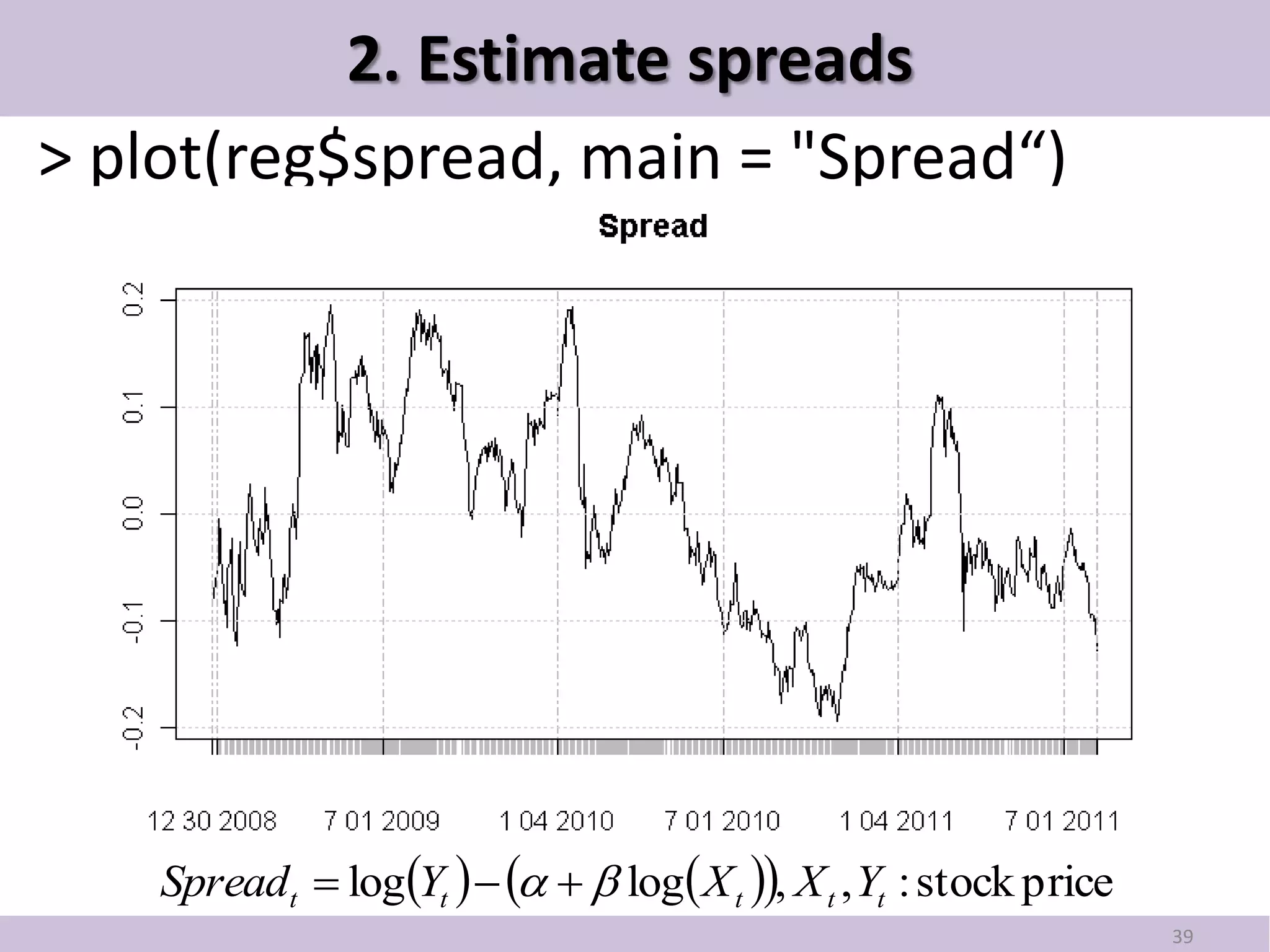
![2. Estimate spreads
> reg <- EstimateParameters(price.pair, method = lm)
> str(reg)
List of 3
$ spread :An ‘xts’ object from 2008-12-30 to 2011-08-05 containing:
Data: num [1:635, 1] -0.08544 -0.0539 -0.04306 -0.00426 -0.01966 ...
- attr(*, "dimnames")=List of 2
..$ : NULL
..$ : chr "B"
Indexed by objects of class: [Date] TZ:
xts Attributes:
NULL
$ hedge.ratio: num 0.0997
$ premium : num 7.48
38](https://image.slidesharecdn.com/introductiontopairtrading-111024073506-phpapp02/75/Introduction-to-pairtrading-38-2048.jpg)


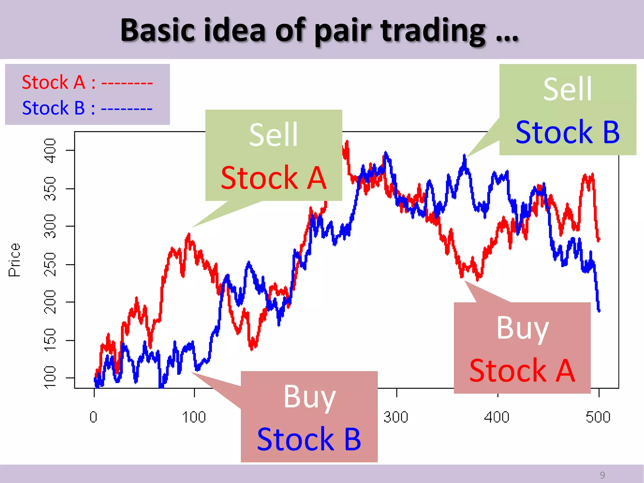
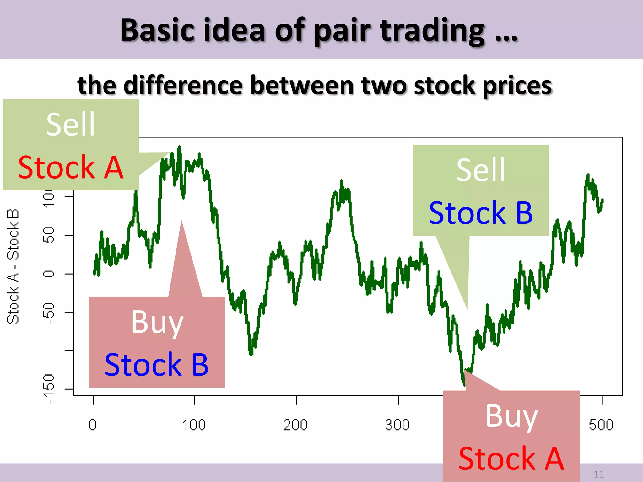
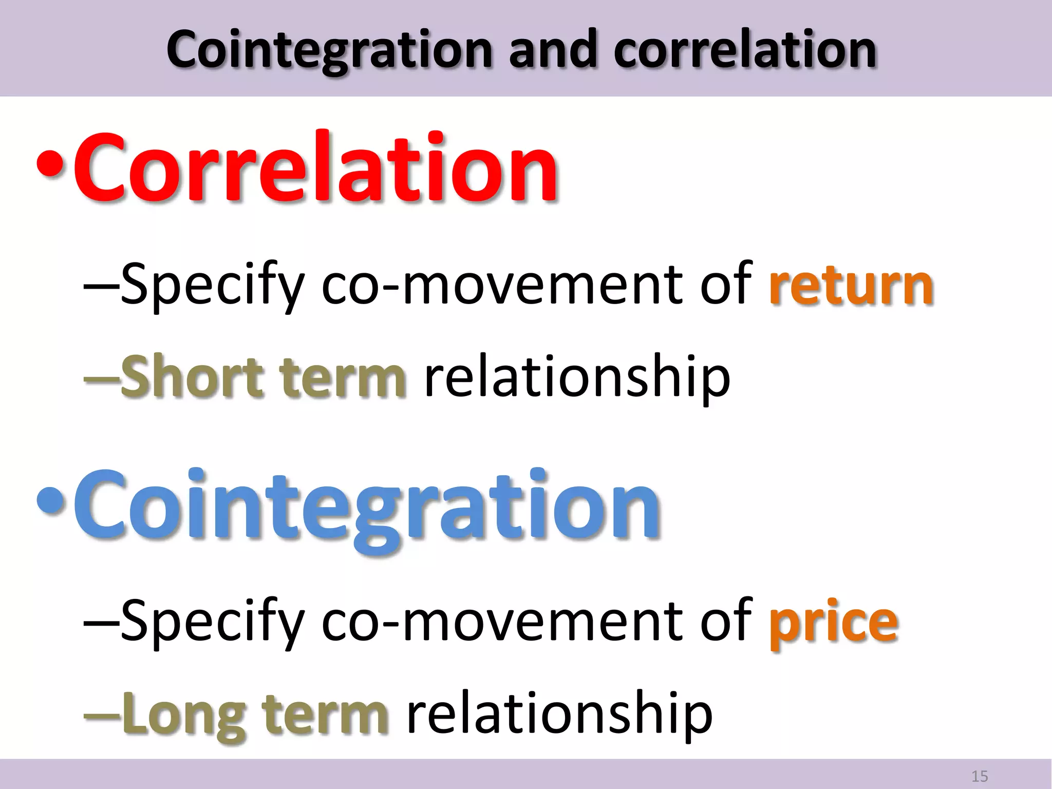
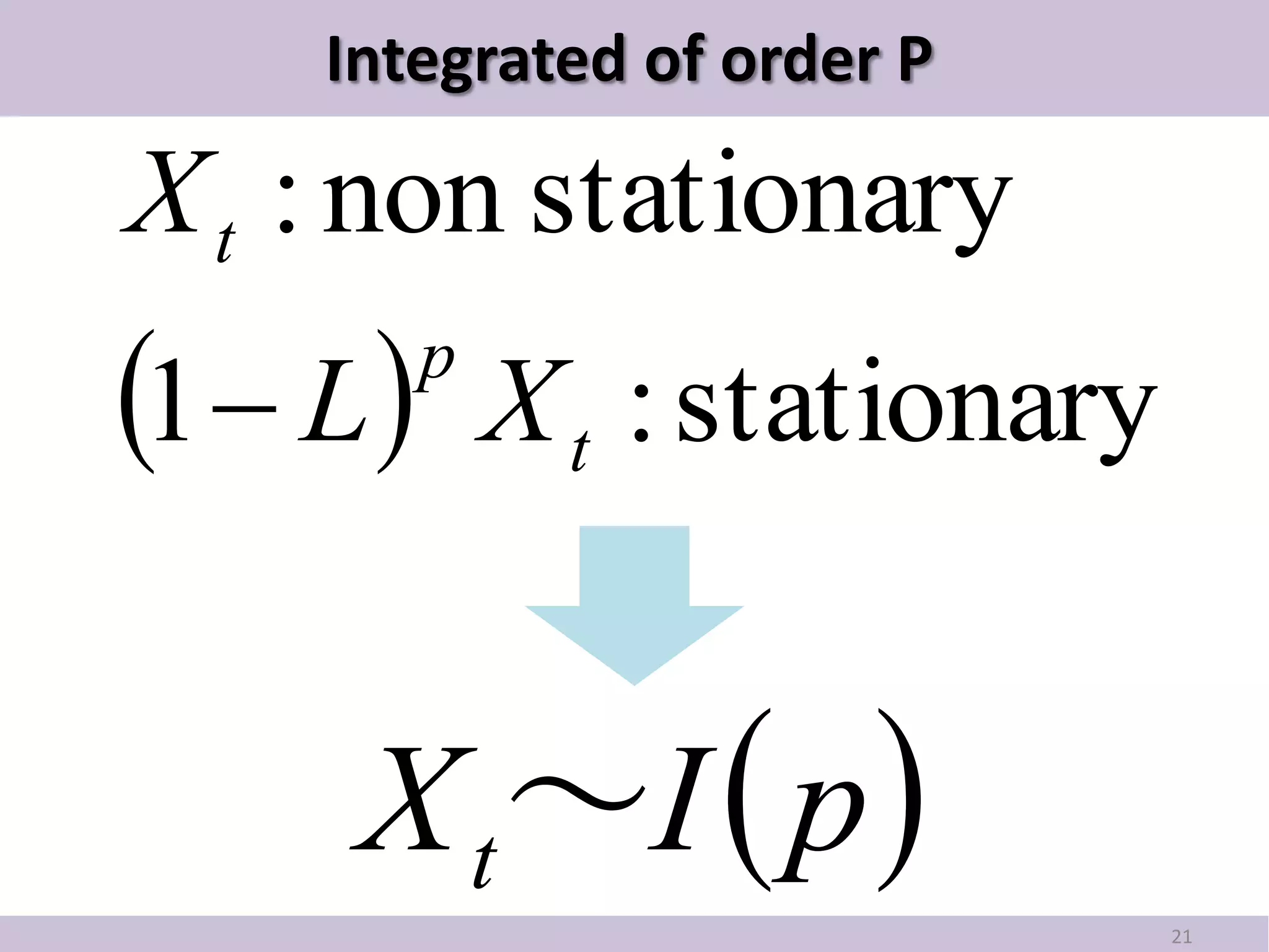
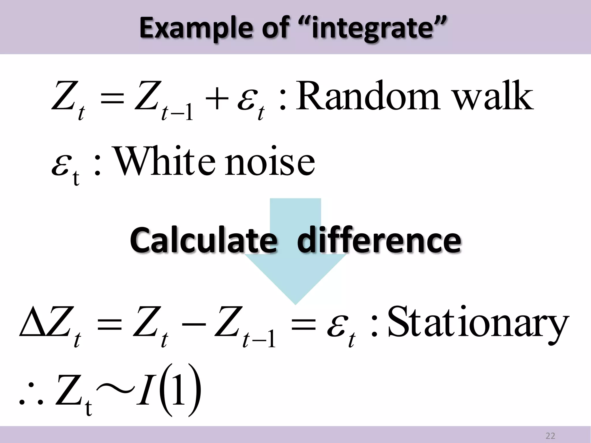
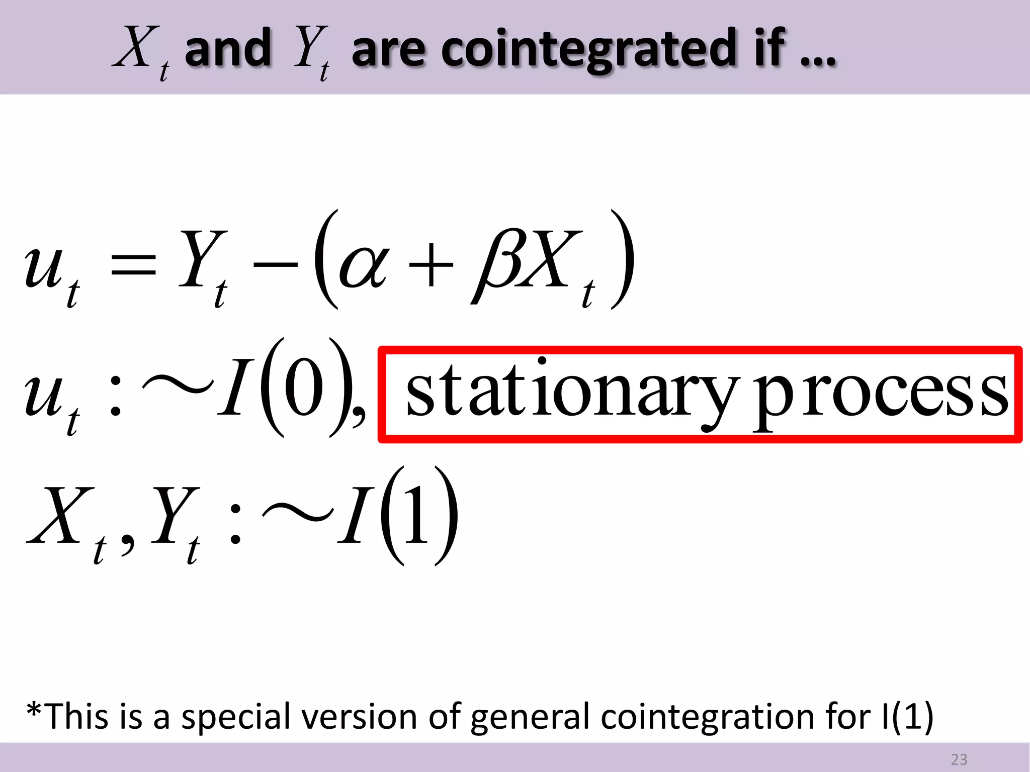
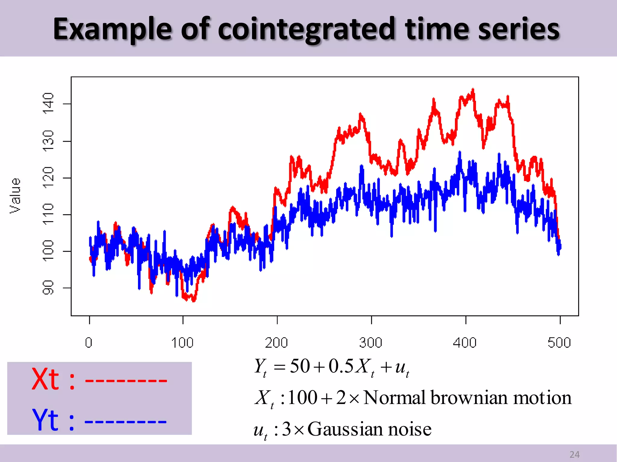
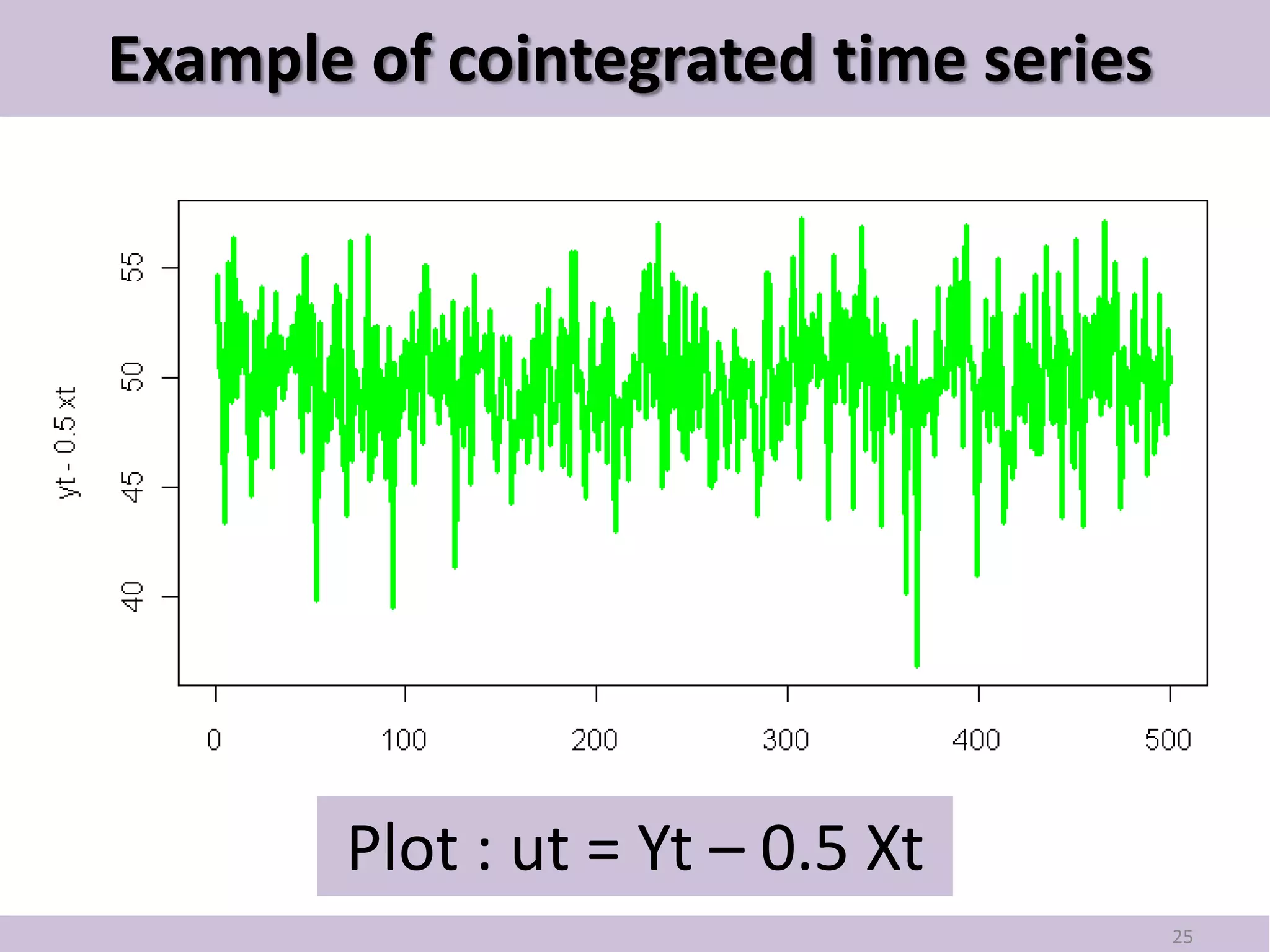
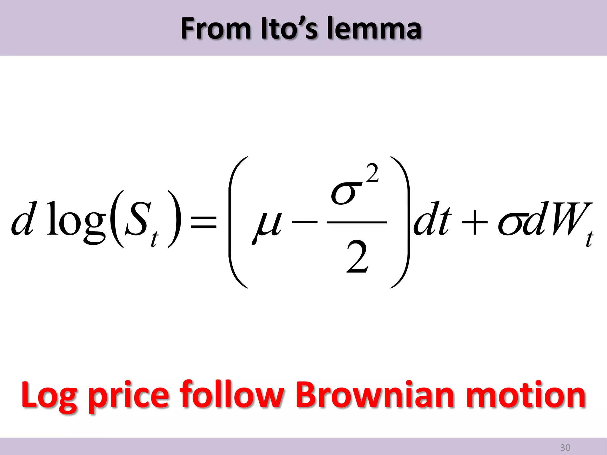
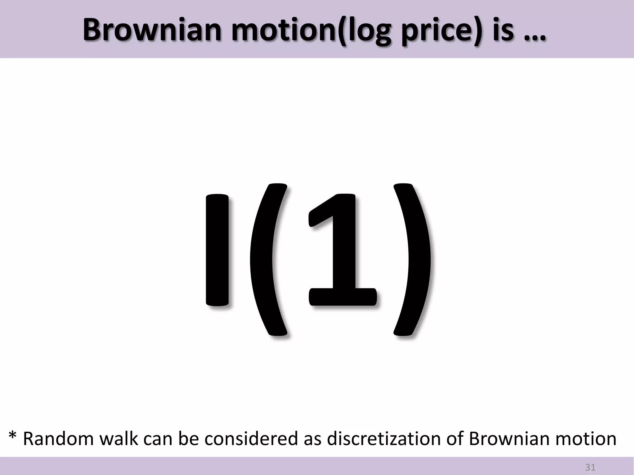
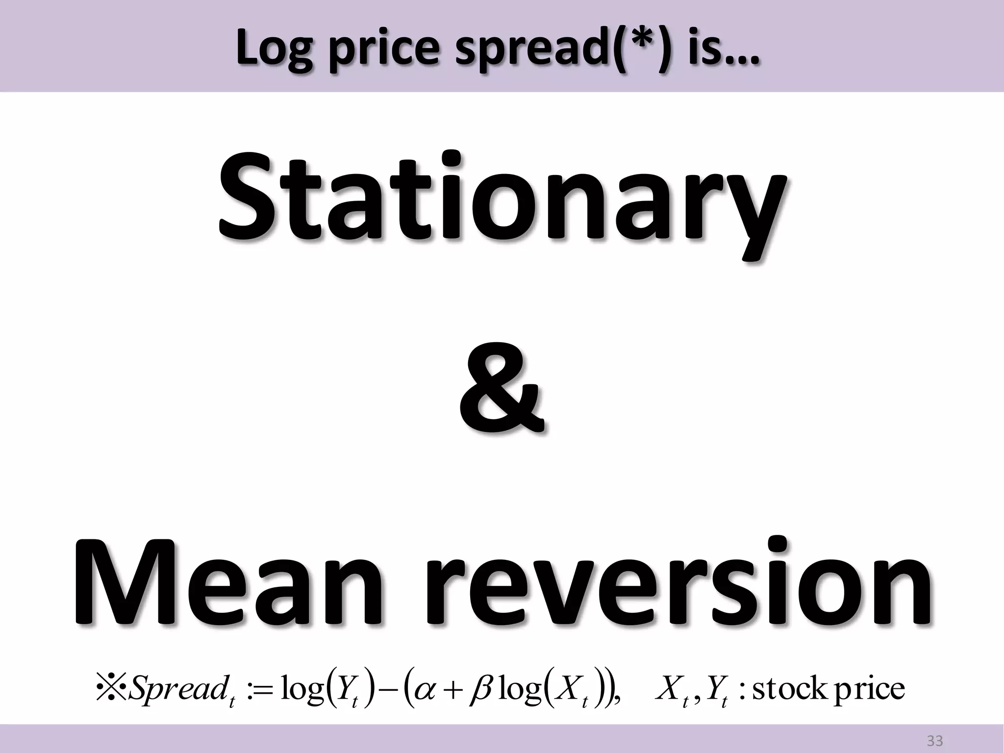
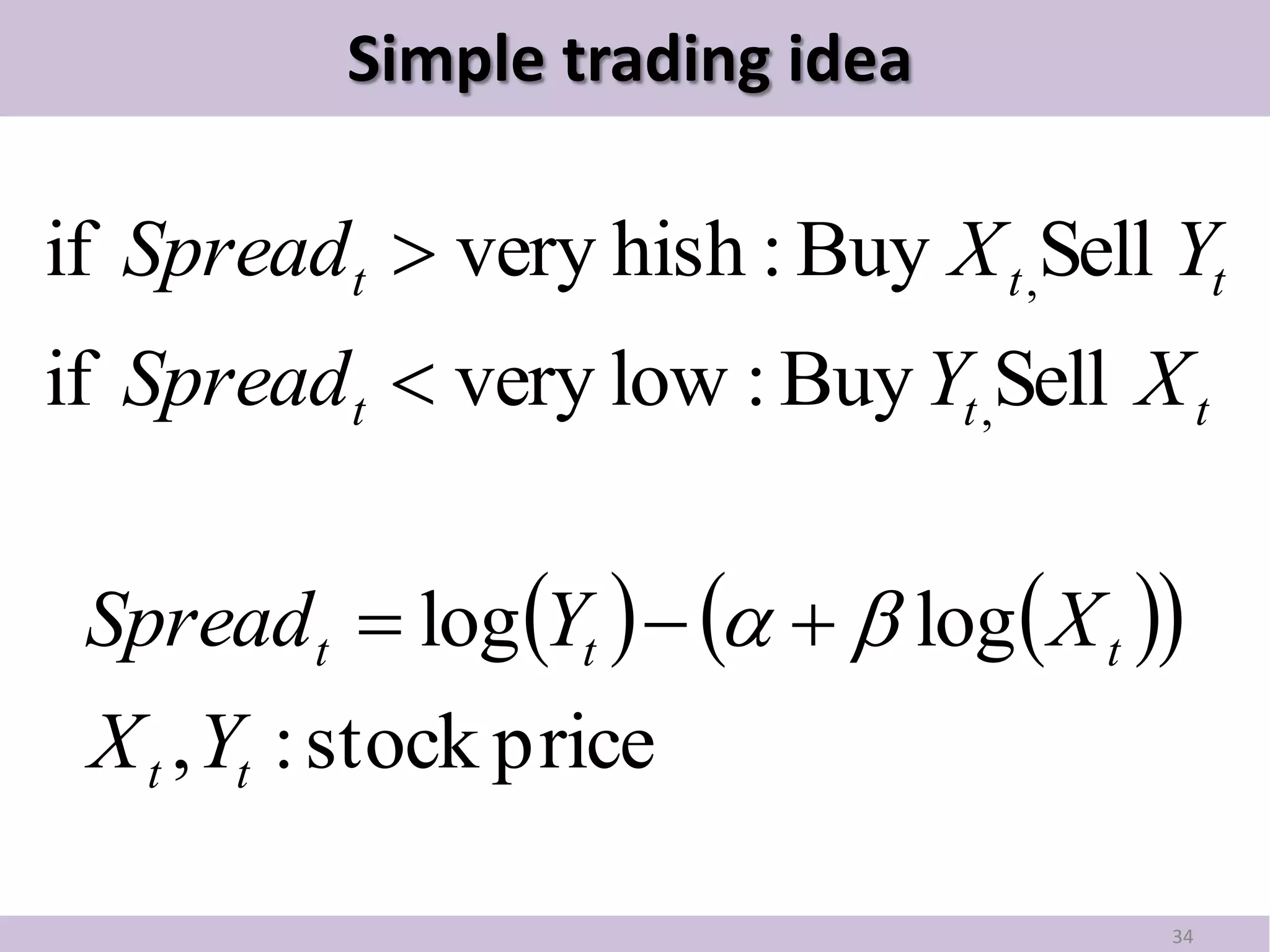
This document provides an introduction to pair trading based on cointegration. It discusses that pair trading selects two highly correlated stocks and trades their price differences. Cointegration refers to the long-term co-movement of stock prices, which pair trading exploits. The document outlines the basic idea of pair trading when stock prices diverge, and simulates pair trading using R language to estimate spreads, check for cointegration, generate signals, and backtest performance. In summary, pair trading is a quantitative strategy that aims to profit from mean reversion of cointegrated stock price spreads.


![[Paper reading] Hamiltonian Neural Networks](https://cdn.slidesharecdn.com/ss_thumbnails/hamiltoniannn-200131102421-thumbnail.jpg?width=640&height=640&fit=bounds)


