1. The document examines the condition for constructing a one-proportion z-interval that np and n(1-p) should each be greater than or equal to 10. It discusses what happens when this condition is violated through simulations.
2. The simulations showed that when n=20 and p=0.1 (violating the condition), the percentage of intervals capturing the true population proportion p of 0.1 was less than the stated 95% confidence level.
3. There are alternative interval construction methods that better match the claimed confidence level when the original condition is violated, such as using an adjusted sample proportion.
1. AP Statistics Name
Why Should np and n(1-p) Be ≥ 10?
A mayoral candidate is interested in what proportion (p) of a large city’s population is planning to
vote for him. Consider our population to be all registered voters in the city. A statistically minded
member of his staff plans to take a simple random sample of all registered voters in the city and get
an estimate of this population proportion.
Once a sample proportion of those who favor the candidate is obtained, performing a One-
Proportion Z-Interval would be a common statistical method to use. This handout examines one
of the conditions required for using that interval and what goes wrong when that condition is
violated.
The condition this handout will examine is the following (n represents the sample size and p
represents the proportion of the population with the desired characteristic).
When constructing a One-Proportion Z-Interval,
np and n (1- p) should each be ≥ 10.
Of course, if you are constructing an interval, then you do not know p (if you knew p, there would
be no reason to construct the interval). Our best check of this condition, then, is to use the sample
ˆ
proportion, p , to check this condition.
What happens when the above condition is violated? What exactly goes wrong? We will simulate
to find out.
VIOLATE THE CONDITION…BUT STILL CONSTRUCT THE INTERVAL
Assume that only 10% of all registered voters in the city plan to vote for the mayoral candidate,
and his staff takes a simple random sample of 20 voters. Thus, n = 20 and p = 0.1 (and np = 2).
You will simulate the process of sampling from this population, then you will make a confidence
interval, and then determine if your interval captures the value of p assumed.
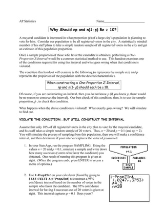
1. In your StatsApp, run the program SAMPLING. Using the
values n = 20 and p = 0.1, simulate a sample and write down
how many successes (voters who favor the candidate) you
obtained. One result of running this program is given at
right. (When the program ends, press ENTER to access a
menu of options.)
2. Use 1- Pr o pZ Int on your calculator (found by going to
STA T : TE S TS - A : 1 - Pr o pZint ) to construct a 95%
confidence interval based on the number of voters in the
sample who favor the candidate. The 95% confidence
interval for having 4 successes out of 20 voters is given at
right. This interval captures p = 0.1 Does yours?
2. Since p = 0.1 was assumed to be the population proportion, we would hope that all our intervals
would capture 0.1. However, we constructed a 95% confidence interval, which means that we
would expect that in the long run 95% of all intervals constructed in the same manner to capture
0.1 and 5% to not capture 0.1. The thrust of this handout is the following:
Suppose the np ≥ 10 and n (1- p) ≥ 10 conditions are violated.
Do 95% confidence intervals still perform as advertised?
One way to determine if in fact the long run proportion of 95% confidence intervals that capture
p = 0.1 is actually 95% is to simulate more intervals.
SIMULATING MORE INTERVALS
3. Run program SAMPLING again. Use n = 20 and p = 0.1 and generate the results for 10
different samples. Record the number of voters who favor the candidate in the table below.
Sample 1 2 3 4 5 6 7 8 9 10
Number of Voters
Favoring Candidate
Does the interval
capture 0.1?
4. For each of the 10 samples above, make a 95% confidence interval using 1- Pr o pZ Int .
Check whether or not each interval captures 0.1 and fill in the above table.
5. Combine your results with your classmates. What percentage of all the computed 95%
confidence intervals captured p = 0.1? Comment on how this percentage compares to the
method’s stated 95% confidence level.
SIMULATING MANY MORE INTERVALS
Of course, simulating even more intervals would give us a better
estimate of the actual “capture rate” for 95% confidence intervals
when n = 20 and p = 0.1.
In your StatsApp, run the program CONFSIML and simulate 100
confidence intervals with n = 20 and p = 0.1. A picture of the
program in progress is given at right.
6. What percentage of your 100 intervals captured p = 0.1? Combine your results with your
classmates. How do your results compare to the stated 95% confidence level?
3. CONSEQUENCES OF VIOLATING THE CONDITION
On the previous page, you most likely found that the percentage of your 100 intervals that captured
p = 0.1 was less than 95%. In fact, the actual capture rate for 95% confidence intervals when
n = 20 and p = 0.1 is only 87.6%. Thus, for this particular combination of n and p, the 95%
confidence interval method will not perform as advertised!
This is why we check the conditions np ≥ 10 and n(1- p) ≥ 10. If either of these conditions is not
true, we run the severe risk of constructing a confidence interval that does not match the method’s
stated confidence level.
7. The table below lists actual confidence interval capture percentages for various
combinations of n and p. Circle the values for which the conditions np ≥ 10 and
n(1- p) ≥ 10 are met.
95% Confidence Interval Capture Percentages
for different combinations of n and p
0.9 65.0% 87.6% 80.9% 91.4% 87.9% … 94.3%
0.8 88.6% 92.1% 94.6% 90.5% 93.8% … 94.9%
0.7 84.0% 94.7% 95.3% 93.0% 93.5% … 94.9%
0.6 89.9% 92.8% 93.5% 94.6% 94.1% … 95.0%
p 0.5 89.1% 95.9% 95.7% 91.9% 93.5% … 94.6%
0.4 89.9% 92.8% 93.5% 94.6% 94.1% … 95.0%
0.3 84.0% 94.7% 95.3% 93.0% 93.5% … 94.9%
0.2 88.6% 92.1% 94.6% 90.5% 93.8% … 94.9%
0.1 65.0% 87.6% 80.9% 91.4% 87.9% … 94.3%
10 20 30 40 50 … 500
n
8. Comment on how the confidence interval capture rate varies for various values of n and p.
4. ARE THERE OTHER OPTIONS?
As you have seen, the traditional One-Proportion Z-Interval usually does not perform as promised
when the conditions np ≥ 10 and n(1- p) ≥ 10 are violated. In fact, there are times when the
interval does not perform as advertised even when the conditions are satisfied – you may have
noticed some of these instances in the table you just examined.
Statisticians are well aware of the deficiencies of the traditional One-Proportion Z-Interval and
have come up with alternative interval making procedures to more closely match the claimed
confidence level. One method adds 2 to the number of successes in the sample and 2 to the
number of failures in the sample to obtain an adjusted value for the sample proportion that is given
x+2
by the formula p =! !
where x is the number of successes. This value of p is then used instead
n+4
ˆ
of p in the traditional One-Proportion Z-Interval. Using this adjusted sample proportion gives
capture percentages that more closely match the advertised confidence level.
The table at right gives the USING THE ADJUSTED SAMPLE PROPORTION
coverage percentages for 95% Confidence Interval Capture Percentages
for different combinations of n and p
various combinations of n
and p using the adjusted 0.9 93.0% 95.7% 97.4% 95.8% 97.0% … 95.6%
sample proportion.
0.8 96.7% 95.6% 96.4% 94.9% 95.1% … 95.0%
9. Circle the capture 0.7 95.3% 97.5% 95.1% 94.4% 95.7% … 95.5%
percentages that are
greater than or equal to 0.6 98.2% 96.3% 96.2% 96.6% 94.1% … 95.0%
95%.
0.5 97.9% 95.9% 95.7% 96.2% 93.5% … 94.6%
(Note this method is still 0.4 98.2% 96.3% 96.2% 96.6% 94.1% … 95.0%
not perfect…but it is an
improvement.) 0.3 95.3% 97.5% 95.1% 94.4% 95.7% … 95.5%
0.2 96.7% 95.6% 96.4% 94.9% 95.1% … 95.0%
0.1 93.0% 95.7% 97.4% 95.8% 97.0% … 95.6%
10 20 30 40 50 … 500
n
There is an applet, written by statisticians Beth Chance and Allan Rossman, which simulates the
making of confidence intervals for any confidence level and any combination of n and p. It is ideal
for further exploration of this issue and can be found at the following address:
http://www.rossmanchance.com/applets/Confsim/Confsim.html
The traditional One-Proportion Z-Interval is named the “Wald” interval in the applet. The method
!
using p is named the “Adjusted Wald” interval. It is interesting to experiment with different
values of n and p for each type of interval.