1. Mining Association Rules with Item Constraints
Ramakrishnan Srikant Quoc Vu Rakesh Agrawal
and and
IBM Almaden Research Center
650 Harry Road, San Jose, CA 95120, U.S.A.
fsrikant,qvu,ragrawalg@almaden.ibm.com
Abstract predicting telecommunications order failures and med-
ical test results. There has been considerable work on
The problem of discovering association rules has re- developing fast algorithms for mining association rules,
ceived considerable research attention and several fast
including Agrawal et al. 1996 Savasere, Omiecinski,
algorithms for mining association rules have been de-
Navathe 1995 Toivonen 1996 Agrawal Shafer
veloped. In practice, users are often interested in a
1996 Han, Karypis, Kumar 1997.
subset of association rules. For example, they may
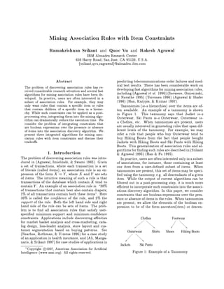
Taxonomies is-a hierarchies over the items are of-
only want rules that contain a speci c item or rules
that contain children of a speci c item in a hierar- ten available. An example of a taxonomy is shown
chy. While such constraints can be applied as a post- in Figure 1. This taxonomy says that Jacket is-a
processing step, integrating them into the mining algo- Outerwear, Ski Pants is-a Outerwear, Outerwear is-
rithm can dramatically reduce the execution time. We a Clothes, etc. When taxonomies are present, users
consider the problem of integrating constraints that
are usually interested in generating rules that span dif-
are boolean expressions over the presence or absence
ferent levels of the taxonomy. For example, we may
of items into the association discovery algorithm. We
infer a rule that people who buy Outerwear tend to
present three integrated algorithms for mining asso-
buy Hiking Boots from the fact that people bought
ciation rules with item constraints and discuss their
Jackets with Hiking Boots and Ski Pants with Hiking
tradeo s.
Boots. This generalization of association rules and al-
gorithms for nding such rules are described in Srikant
1. Introduction Agrawal 1995 Han Fu 1995.
The problem of discovering association rules was intro- In practice, users are often interested only in a subset
duced in Agrawal, Imielinski, Swami 1993. Given of associations, for instance, those containing at least
a set of transactions, where each transaction is a set one item from a user-de ned subset of items. When
of literals called items, an association rule is an ex- taxonomies are present, this set of items may be speci-
pression of the form X Y , where X and Y are sets ed using the taxonomy, e.g. all descendants of a given
of items. The intuitive meaning of such a rule is that item. While the output of current algorithms can be
transactions of the database which contain X tend to ltered out in a post-processing step, it is much more
contain Y . An example of an association rule is: 30 e cient to incorporate such constraints into the associ-
of transactions that contain beer also contain diapers; ations discovery algorithm. In this paper, we consider
2 of all transactions contain both these itemsquot;. Here constraints that are boolean expressions over the pres-
30 is called the con dence of the rule, and 2 the ence or absence of items in the rules. When taxonomies
support of the rule. Both the left hand side and right are present, we allow the elements of the boolean ex-
hand side of the rule can be sets of items. The prob- pression to be of the form ancestorsitem or descen-
lem is to nd all association rules that satisfy user-
speci ed minimum support and minimum con dence
constraints. Applications include discovering a nities Clothes Footwear
for market basket analysis and cross-marketing, cata-
log design, loss-leader analysis, store layout and cus-
tomer segmentation based on buying patterns. See Outerwear Shirts Shoes Hiking Boots
Nearhos, Rothman, Viveros 1996 for a case study
of an application in health insurance, and Ali, Manga-
naris, Srikant 1997 for case studies of applications in
Jackets Ski Pants
Copyright c 1997, American Association for Arti cial
1
Figure 1: Example of a Taxonomy
Intelligence www.aaai.org. All rights reserved.

2. : descendantlij . There is no bound on the num-
dantsitem rather than just a single item. For exam-
ple, ber of ancestors or descendants that can be included.
To evaluate B, we implicitly replace descendantlij
Jacket ^ Shoes _ descendantsClothes ^ 0 00
by lij _ lij _ lij _ : : :, and : descendantlij by
: ancestorsHiking Boots 0 _l00 _: : :, where l0 ; l00 ; : : : are the descendants
:lij _lij ij ij ij
expresses the constraint that we want any rules that of lij . We perform a similar operation for ancestor.
either a contain both Jackets and Shoes, or b con- To evaluate B over a rule X Y , we consider all items
tain Clothes or any descendants of clothes and do not that appear in X Y to have a value true in B and
contain Hiking Boots or Footwear. all other items to have a value false.
Given a set of transactions D, a set of taxonomies
Paper Organization We give a formal description G and a boolean expression B, the problem of mining
of the problem in Section 2. Next, we review the Apri- association rules with item constraints is to discover all
ori algorithm Agrawal et al. 1996 for mining associ- rules that satisfy B and have support and con dence
ation rules in Section 3. We use this algorithm as the greater than or equal to the user-speci ed minimum
basis for presenting the three integrated algorithms for support and minimum con dence respectively.
mining associations with item constraints in Section 4.
3. Review of Apriori Algorithm
However, our techniques apply to other algorithms that
use apriori candidate generation, including the recently The problem of mining association rules can be decom-
published Toivonen 1996. We discuss the tradeo s posed into two subproblems:
between the algorithms in Section 5, and conclude with
Find all combinations of items whose support is
a summary in Section 6.
greater than minimum support. Call those combi-
2. Problem Statement nations frequent itemsets.
Use the frequent itemsets to generate the desired
Let L = fl1; l2 ; : : :; lm g be a set of literals, called items.
rules. The general idea is that if, say, ABCD and
Let G be a directed acyclic graph on the literals. An
AB are frequent itemsets, then we can determine if
edge in G represents an is-a relationship, and G repre-
the rule AB CD holds by computing the ratio r =
sents a set of taxonomies. If there is an edge in G from
supportABCD supportAB. The rule holds only
p to c, we call p a parent of c and c a child of p p rep-
if r minimum con dence. Note that the rule will
resents a generalization of c. We call x an ancestor of
have minimum support because ABCD is frequent.
y and y a descendant of x if there is a directed path
from x to y in G. We now present the Apriori algorithm for nding all
Let D be a set of transactions, where each transac- frequent itemsets Agrawal et al. 1996. We will use
tion T is a set of items such that T

3. L. We say that this algorithm as the basis for our presentation. Let
a transaction T supports an item x 2 L if x is in T k-itemset denote an itemset having k items. Let Lk
or x is an ancestor of some item in T . We say that a represent the set of frequent k-itemsets, and Ck the
transaction T supports an itemset X

4. L if T supports set of candidate k-itemsets potentially frequent item-
every item in the set X. sets. The algorithm makes multiple passes over the
A generalized association rule is an implication of data. Each pass consists of two phases. First, the
the form X Y , where X L, Y L, X Y = ;.1 set of all frequent k,1-itemsets, Lk,1, found in the
The rule X Y holds in the transaction set D with k,1th pass, is used to generate the candidate itemsets
con dence c if c of transactions in D that support X Ck . The candidate generation procedure ensures that
also support Y . The rule X Y has support s in the Ck is a superset of the set of all frequent k-itemsets.
transaction set D if s of transactions in D support The algorithm now scans the data. For each record, it
X Y. determines which of the candidates in Ck are contained
Let B be a boolean expression over L. We as- in the record using a hash-tree data structure and in-
sume without loss of generality that B is in disjunc- crements their support count. At the end of the pass,
tive normal form DNF.2 That is, B is of the form Ck is examined to determine which of the candidates
D1 _D2 _: : :_Dm , where each disjunct Di is of the form are frequent, yielding Lk . The algorithm terminates
i1 ^ i2 ^ : : : ^ in . When there are no taxonomies when Lk becomes empty.
present, each element ij is either lij or :lij for some
i
lij 2 L. When a taxonomy G is present, ij can also Candidate Generation Given Lk , the set of all fre-
be ancestorlij , descendantlij, : ancestorlij , or quent k-itemsets, the candidate generation procedure
returns a superset of the set of all frequent k + 1-
Usually, we also impose the condition that no item in
1
itemsets. We assume that the items in an itemset are
Y should be an ancestor of any item in X. Such a rule
lexicographically ordered. The intuition behind this
would have the same support and con dence as the rule
procedure is that all subsets of a frequent itemset are
without the ancestor in Y , and is hence redundant.
also frequent. The function works as follows. First, in
Any boolean expression can be converted to a DNF
2
the join step, Lk is joined with itself:
expression.

5. Phase 2 To generate rules from these frequent item-
C
insert into k+1
p:item ; p:item2 ; : : :; p:itemk ; q:itemk sets, we also need to nd the support of all subsets of
1
select
frequent itemsets that do not satisfy B. Recall that
L p, L q
from k k
to generate a rule AB CD, we need the support
p:item = q:item1; : : :; p:itemk,1 = q:itemk,1;
1
where
p:itemk q:itemk ; of AB to nd the con dence of the rule. However,
AB may not satisfy B and hence may not have been
Next, in the prune step, all itemsets c 2 Ck+1, where counted in Phase 1. So we generate all subsets of the
some k-subset of c is not in Lk , are deleted. A proof frequent itemsets found in Phase 1, and then make
of correctness of the candidate generation procedure is an extra pass over the dataset to count the support
given in Agrawal et al. 1996. of those subsets that are not present in the output
We illustrate the above steps with an example. Let of Phase 1.
L3 be ff1 2 3g, f1 2 4g, f1 3 4g, f1 3 5g, f2 3 4gg. After
Phase 3 Generate rules from the frequent itemsets
the join step, C4 will be ff1 2 3 4g, f1 3 4 5gg. The
found in Phase 1, using the frequent itemsets found
prune step will delete the itemset f1 3 4 5g because
in Phases 1 and 2 to compute con dences, as in the
the subset f1 4 5g is not in L3. We will then be left
Apriori algorithm.
with only f1 2 3 4g in C4 .
Notice that this procedure is no longer complete We discuss next the techniques for nding frequent
when item constraints are present: some candidates itemsets that satisfy B Phase 1. The algorithms use
that are frequent will not be generated. For example, the notation in Figure 2.
let the item constraint be that we want rules that con-
4.1 Approaches using Selected Items
tain the item 2, and let L2 = f f1 2g, f2 3g g. For
the Apriori join step to generate f1 2 3g as a candi- Generating Selected Items Recall the boolean
date, both f1 2g and f1 3g must be present but f1 expression B = D1 _ D2 _ : : : _ Dm , where Di =
3g does not contain 2 and will not be counted in the i1 ^ i2 ^ : : : ^ in and each element ij is either
second pass. We discuss various algorithms for candi- lij or :lij , for some lij 2 L. We want to generate a set
i
date generation in the presence of constraints in the of items S such that any itemset that satis es B will
next section. contain at least one item from S. For example, let the
set of items L = f1; 2; 3; 4;5g. Consider B = 1^2_3.
4. Algorithms The sets f1, 3g, f2, 3g and f1, 2, 3, 4, 5g all have the
property that any non-empty itemset that satis es B
We rst present the algorithms without considering
will contain an item from this set. If B = 1 ^ 2 _ :3,
taxonomies over the items in Sections 4.1 and 4.2, and
the set f1, 2, 4, 5g has this property. Note that the
then discuss taxonomies in Section 4.3. We split the
inverse does not hold: there are many itemsets that
problem into three phases:
contain an item from S but do not satisfy B.
Phase 1 Find all frequent itemsets itemsets whose For a given expression B, there may be many di er-
support is greater than minimum support that sat- ent sets S such that any itemset that satis es B con-
isfy the boolean expression B. Recall that there are tains an item from S. We would like to choose a set of
two types of operations used for this problem: can- items for S so that the sum of the supports of items in
didate generation and counting support. The tech- S is minimized. The intuition is that the sum of the
niques for counting the support of candidates remain supports of the items is correlated with the sum of the
unchanged. However, as mentioned above, the apri- supports of the frequent itemsets that contain these
ori candidate generation procedure will no longer items, which is correlated with the execution time.
generate all the potentially frequent itemsets as can- We now show that we can generate S by choosing
didates when item constraints are present. one element ij from each disjunct Di in B, and adding
We consider three di erent approaches to this prob- either lij or all the elements in L , flij g to S, based
lem. The rst two approaches, MultipleJoinsquot; and on whether ij is lij or :lij respectively. We de ne an
Reorderquot;, share the following approach Section element ij = lij in B to be presentquot; in S if lij 2 S
4.1: and an element ij = :lij to be presentquot; if all the
1. Generate a set of selected items S such that any items in L , flij g are in S. Then:
itemset that satis es B will contain at least one Lemma 1 Let S be a set of items such that
selected item.
8Di 2 B 9 ij 2 Di ij = lij ^ lij 2 S _
2. Modify the candidate generation procedure to
ij = :lij ^ L , flij g

6. S :
only count candidates that contain selected items.
3. Discard frequent itemsets that do not satisfy B. Then any non-empty itemset that satis es B will con-
tain an item in S.
The third approach, Directquot; directly uses the
Proof: Let X be an itemset that satis es B. Since X
boolean expression B to modify the candidate gener-
satis es B, there exists some Di 2 B that is true for X.
ation procedure so that only candidates that satisfy
B are counted Section 4.2. From the lemma statement, there exists some ij 2 Di

7. B = D1 _ D2 _ : : : _ Dm m disjuncts
Di = i1 ^ i2 ^ : : : ^ in ni conjuncts in Di
i
ij is either lij or :lij , for some item lij 2 L
S Set of items such that any itemset that satis es B contains an item from S
selected itemset An itemset that contains an item in S
k-itemset An itemset with k items.
Ls Set of frequent k-itemsets those with minimum support that contain an item in S
k
Lb Set of frequent k-itemsets those with minimum support that satisfy B
k
s
Ck Set of candidate k-itemsets potentially frequent itemsets that contain an item in S
b
Ck Set of candidate k-itemsets potentially frequent itemsets that satisfy B
F Set of all frequent items
Figure 2: Notation for Algorithms
such that either ij = lij and lij 2 S or ij = :lij and procedure must return a superset of the set of all se-
L , flij g

8. S. If the former, we are done: since Di lected frequent k+1-itemsets.
is true for X, lij 2 X. If the latter, X must contain Recall that unlike in the Apriori algorithm, not all
some item in in L , flij g since X does not contain lij s s
subsets of candidates in Ck+1 will be in Lk . While
and X is not an empty set. Since L , flij g

9. S, X all subsets of a frequent selected itemset are frequent,
contains an item from S. 2 they may not be selected itemsets. Hence the join pro-
cedure of the Apriori algorithm will not generate all
A naive optimal algorithm for computing the set of the candidates.
Qi=1
elements in S such that supportS is minimum would
To generate C2 we simply take Ls F, where F is
s
require m ni time, where ni is the number of con- 1
the set of all frequent items. For subsequent passes,
P is
juncts in the disjunct Di . An alternativem the fol-
one solution would be to join any two elements of Ls
lowing greedy algorithm which requires i=1 ni time k
that have k,1 items in common. For any selected k-
and is optimal if no literal is present more than once
itemset where k 2, there will be at least 2 subsets
in B. We de ne S ij to be S lij if ij = lij and
with a selected item: hence this join will generate all
S L , flij g if ij = :lij . the candidates. However, each k + 1-candidate may
S := ;; have up to k frequent selected k-subsets and kk,1
B = D1 _ D2 _ : : : _ Dm
for i := 1 to m do begin pairs of frequent k-subsets with k ,1 common items.
Di = i1 ^ i2 ^ : : : ^ in
for j := 1 to ni do Hence this solution can be quite expensive if there are
Cost ij := supportS ij - supportS;
i
a large number of itemsets in Ls .
k
Let ip be the ij with the minimum cost. We now present two more e cient approaches.
S := S ip;
Algorithm MultipleJoins The following lemma
end
presents the intuition behind the algorithm. The item-
Consider a boolean expression B where the same lit- set X in the lemma corresponds to a candidate that we
eral is present in di erent disjuncts. For example, let need to generate. Recall that the items in an itemset
B = 1 ^ 2 _ 1 ^ 3. Assume 1 has higher support are lexicographically ordered.
than 2 or 3. Then the greedy algorithm will generate
Lemma 2 Let X be a frequent k+1-itemset, k 2.
S = f2; 3g whereas S = f1g is optimal. A partial x for
A. If X has a selected item in the rst k,1 items,
this problem would be to add the following check. For
then there exist two frequent selected k-subsets of X
each literal lij that is present in di erent disjuncts, we
add lij to S and remove any redundant elements from with the same rst k,1 items as X.
B. If X has a selected item in the last mink ,1, 2
S, if such an operation would decrease the support of
S. If there are no overlapping duplicates two dupli- items, then there exist two frequent selected k-subsets
cated literals in the same disjunct, this will result in of X with the same last k,1 items as X.
C. If X is a 3-itemset and the second item is a se-
the optimal set of items. When there are overlapping
duplicates, e.g, 1 ^ 2 _ 1 ^ 3 _ 3 ^ 4, the algorithm lected item, then there exist two frequent selected 2-
may choose f1; 4g even if f2; 3g is optimal. subsets of X, Y and Z, such that the last item of Y
Next, we consider the problem of generating only is the second item of X and the rst item of Z is the
those candidates that contain an item in S. second item of X.
Candidate Generation Given Ls , the set of all se- For example, consider the frequent 4-itemset f1 2 3
k
4g. If either 1 or 2 is selected, f1 2 3g and f1 2 4g are
lected frequent k-itemsets, the candidate generation

10. Ls 0 Ls 00 Join 1 Join 2 Join 3
two subsets with the same rst 2 items. If either 3 or 2 2
f2 3g f1 2g f2 3 5g f1 2 3g
4 is selected, f2 3 4g and f1 3 4g are two subsets with
f2 5g f1 4g f1 3 4g f1 2 5g
the same last 2 items. For a frequent 3-itemset f1 2 3g
f3 4g
where 2 is the only selected item, f1 2g and f2 3g are
the only two frequent selected subsets.
Figure 3: MultipleJoins Example
Generating an e cient join algorithm is now
straightforward: Joins 1 through 3 below correspond
Ls Join 1
directly to the three cases in the lemma. Consider a 2
f2 1g f2 1 3g
candidate k+1-itemset X, k 2. In the rst case,
f2 3g f2 1 5g
Join 1 below will generate X. Join 1 is similar to
f2 5g f2 3 5g
the join step of the Apriori algorithm, except that it is
f4 1g f4 1 3g
performed on a subset of the itemsets in Ls . In the
2
f4 3g
second case, Join 2 will generate X. When k 3, we
have covered all possible locations for a selected item
Figure 4: Reorder Example
in X. But when k = 2, we also need Join 3 for the
case where the selected item in X is the second item.
Figure 3 illustrates this algorithm for S = f2, 4g and
procedure of the Apriori algorithm applied to Ls will
an Ls with 4 itemsets. k
2
generate a superset of Ls .
k+1
Join 1
Ls 0 := fp 2 Ls j one of the rst k,1 items of p is in Sg The intuition behind this lemma is that the rst item
k ks
of any frequent selected itemset is always a selected
insert into Ck+1
item. Hence for any k+1-candidate X, there exist
select p:item1 ; p:item2 ; : : :; p:itemk ; q:itemk
two frequent selected k-subsets of X with the same rst
from Ls 0 p, Ls 0 q
k k k,1 items as X. Figure 4 shows the same example as
where p:item1 = q:item1; : : : ; p:itemk,1 = q:itemk,1;
shown in Figure 3, but with the items in S, 2 and 4,
p:itemk q:itemk
ordered before the other items, and with the Apriori
Join 2 join step.
Ls 00 := fp 2 Ls j one of the last mink ,1,2 items Hence instead of using the lexicographic ordering of
k k
of p is in Sg items in an itemset, we impose the following ordering.
s
insert into Ck+1 All items in S precede all items not in S; the lexico-
select p:item1 ; q:item1; q:item2 ; : : :; q:itemk graphic ordering is used when two items are both in S
from Ls 00 p, Ls 00 q or both not in S. An e cient implementation of an as-
k k
where p:item1 q:item1; p:item2 = q:item2 ; : : : ; sociation rule algorithm would map strings to integers,
p:itemk = q:itemk rather than keep them as strings in the internal data
Join 3 k = s2 structures. This mapping can be re-ordered so that
all the frequent selected items get lower numbers than
insert into C3
other items. After all the frequent itemsets have been
select q:item1 ; p:item1; p:item2
from Ls 0 p, Ls 00 q found, the strings can be re-mapped to their original
2 2
values. One drawback of this approach is that this re-
where q:item2 = p:item1 and
ordering has to be done at several points in the code,
q:item1, p:item2 are not selected;
including the mapping from strings to integers and the
Note that these three joins do not generate any du- data structures that represent the taxonomies.
plicate candidates. The rst k,1 items of any two
candidate resulting from Joins 1 and 2 are di erent. 4.2 Algorithm Direct
When k = 2, the rst and last items of candidates
Instead of rst generating a set of selected items S
resulting from Join 3 are not selected, while the rst
from B, nding all frequent itemsets that contain one
item is selected for candidates resulting from Join 1
or more items from S and then applying B to lter the
and the last item is selected for candidates resulting
frequent itemsets, we can directly use B in the candi-
from Join 1. Hence the results of Join 3 do not overlap
date generation procedure. We rst make a pass over
with either Join 1 or Join 2. b
the data to nd the set of the frequent items F. L1
In the prune step, we drop candidates with a selected
is now the set of those frequent 1-itemsets that sat-
subset that is not present in Ls . k isfy B. The intuition behind the candidate generation
Algorithm Reorder As before, we generate C2 by s procedure is given in the following lemma.
taking Ls F. But we use the following lemma to
1 Lemma 4 For any k +1-itemset X which satis es
simplify the join step. B, there exists at least one k-subset that satis es B
Lemma 3 If the ordering of items in itemsets is such unless each Di which is true on X has exactly k +1
that all items in S precede all items not in S, the join non-negated elements.

11. b b
We generate Ck+1 from Lk in 4 steps: contains both an item and its ancestor will be gen-
erated. For example, an itemset fJacket Outerwear
1. Ck+1 := Lb F;
b
Shoesg would not be generated in C3 because fJacket
k
Outerwearg would have been deleted from L2 . How-
b
2. Delete all candidates in Ck+1 that do not not satisfy
ever, this property does not hold when item constraints
B;
are speci ed. In this case, we need to check each can-
b
3. Delete all candidates in Ck+1 with a k-subset that didate in every pass to ensure that there are no can-
satis es B but does not have minimum support. didates that contain both an item and its ancestor.
4. For each disjunct Di = i1 ^ i2 ^ : : : ^
5. Tradeo s
in in B with exactly k + 1 non-negated el-
ements ip1 ; ip2 ; : : :; ip , add the itemset
i
Reorder and MultipleJoins will have similar perfor-
k+1
b
f ip1 ip2 : : :; ip g to Ck+1 if all the ip s are fre- mance since they count exactly the same set of can-
quent,
k+1 j
didates. Reorder can be a little faster during the
prune step of the candidate generation, since check-
For example, let L = f1; 2; 3; 4; 5g and B = 1 ^ 2 _
ing whether an k-subset contains a selected item takes
4 ^ :5. Assume all the items are frequent. Then
O1 time for Reorder versus Ok time for Multiple-
Lb = ff4gg. To generate C2 , we rst take Lb F to
b
1 1
Joins. However, if most itemsets are small, this di er-
get f f1 4g, f2 4g, f3 4g, f4 5g g. Since f4 5g does
ence in time will not be signi cant. Execution times
b
not satisfy B, it is dropped. Step 3 does not change C2
are typically dominated by the time to count support
since all 1-subsets that satisfy B are frequent. Finally,
of candidates rather than candidate generation. Hence
b
we add f1 2g to C2 to get ff1 2g, f1 4g, f2 4g, f3 4gg.
the slight di erences in performance between Reorder
4.3 Taxonomies and MultipleJoins are not enough to justify choosing
one over the other purely on performance grounds. The
The enhancements to the Apriori algorithm for inte- choice is to be made on whichever one is easier to im-
grating item constraints apply directly to the algo- plement.
rithms for mining association rules with taxonomies Direct has quite di erent properties than Reorder
given in Srikant Agrawal 1995. We discuss the Cu- and MultipleJoins. We illustrate the tradeo s be-
mulate algorithm here.3 This algorithm adds all ances- tween Reorder MultipleJoins and Direct with an ex-
tors of each item in the transaction to the transaction, ample. We use Reorderquot; to characterize both Re-
and then runs the Apriori algorithm over these ex- order and MultipleJoins in the rest of this comparison.
tended transactionsquot;. For example, using the taxon- Let B = 1 ^ 2 and S = f1g. Assume the 1-itemsets
omy in Figure 1, a transaction fJackets, Shoesg would f1g through f100g are frequent, the 2-itemsets f1 2g
be replaced with fJackets, Outerwear, Clothes, Shoes, through f1 5g are frequent, and no 3-itemsets are fre-
Footwearg. Cumulate also performs several optimiza- quent. Reorder will count the ninety-nine 2-itemsets f1
tion, including adding only ancestors which are present 2g through f1 100g, nd that f1 2g through f1 5g are
in one or more candidates to the extended transaction frequent, count the six 3-itemsets f1 2 3g through f1
and not counting any itemset which includes both an 4 5g, and stop. Direct will count f1 2g and the ninety-
item and its ancestor. eight 3-itemsets f1 2 3g through f1 2 100g. Reorder
Since the basic structure and operations of Cumu- counts a total of 101 itemsets versus 99 for Direct, but
late are similar to those of Apriori, we almost get most of those itemsets are 2-itemsets versus 3-itemsets
taxonomies for freequot;. Generating the set of selected for Direct.
items, S is more expensive since for elements in B that If the minimumsupport was lower and f1 2g through
include an ancestor or descendant function, we also f1 20g were frequent, Reorder will count an additional
need to nd the support of the ancestors or descen- 165 19 18=2 , 6 candidates in the third pass. Re-
dants. Checking whether an itemset satis es B is also order can prune more candidates than Direct in the
more expensive since we may need to traverse the hi- fourth and later passes since it has more information
erarchy to nd whether one item is an ancestor of an- about which 3-itemsets are frequent. For example, Re-
other. order can prune the candidate f1 2 3 4g if f1 3 4g
Cumulate does not count any candidates with both was not frequent, whereas Direct never counted f1
an item and its ancestor since the support of such an 3 4g. On the other hand, Direct will only count 4-
itemset would be the same as the support of the item- candidates that satisfy B while Reorder will count any
set without the ancestor. Cumulate only checks for 4-candidates that include 1.
such candidates during the second pass candidates of If B were 1^2^3quot; rather than 1^2quot;, the gap in the
size 2. For subsequent passes, the apriori candidate number of candidates widens a little further. Through
generation procedure ensures that no candidate that the fourth pass, Direct will count 98 candidates: f1 2
3g and f1 2 3 4g through f1 2 3 100g. For the minimum
The other fast algorithm in Srikant Agrawal 1995,
3
support level in the previous paragraph, Reorder will
EstMerge, is similar to Cumulate, but also uses sampling
count 99 candidates in the second pass, 171 candidates
to decrease the number of candidates that are counted.

12. in the third pass, and if f1 2 3g through f1 5 6g were Agrawal, R.; Mannila, H.; Srikant, R.; Toivonen, H.;
frequent candidates, 10 candidates in the fourth pass, and Verkamo, A. I. 1996. Fast Discovery of Asso-
for a total of 181 candidates. ciation Rules. In Fayyad, U. M.; Piatetsky-Shapiro,
G.; Smyth, P.; and Uthurusamy, R., eds., Advances in
Direct will not always count fewer candidates than
Reorder. Let B be 1 ^ 2 ^ 3 _ 1 ^ 4 ^ 5quot; and S be Knowledge Discovery and Data Mining. AAAI MIT
f1g. Let items 1 through 100, as well as f1 2 3g, f1 4 Press. chapter 12, 307 328.
5g and their subsets be the only frequent sets. Then Agrawal, R.; Imielinski, T.; and Swami, A. 1993.
Reorder will count around a hundred candidates while Mining association rules between sets of items in large
Direct will count around two hundred. databases. In Proc. of the ACM SIGMOD Conference
In general, we expect Direct to count fewer candi- on Management of Data, 207 216.
dates than Reorder at low minimum supports. But the Ali, K.; Manganaris, S.; and Srikant, R. 1997. Partial
candidate generation process will be signi cantly more Classi cation using Association Rules. In Proc. of
expensive for Direct, since each subset must be checked the 3rd Int'l Conference on Knowledge Discovery in
against a potentially complex boolean expression in Databases and Data Mining.
the prune phase. Hence Direct may be better at lower Han, J., and Fu, Y. 1995. Discovery of multiple-level
minimum supports or larger datasets, and Reorder for association rules from large databases. In Proc. of the
higher minimum supports or smaller datasets. Fur- 21st Int'l Conference on Very Large Databases.
ther work is needed to analytically characterize these
Han, E.-H.; Karypis, G.; and Kumar, V. 1997. Scal-
trade-o s and empirically verify them.
able parallel data mining for association rules. In
6. Conclusions Proc. of the ACM SIGMOD Conference on Manage-
ment of Data.
We considered the problem of discovering association Nearhos, J.; Rothman, M.; and Viveros, M. 1996.
rules in the presence of constraints that are boolean Applying data mining techniques to a health insur-
expressions over the presence of absence of items. Such ance information system. In Proc. of the 22nd Int'l
constraints allow users to specify the subset of rules Conference on Very Large Databases.
that they are interested in. While such constraints can
Savasere, A.; Omiecinski, E.; and Navathe, S. 1995.
be applied as a post-processing step, integrating them
An e cient algorithm for mining association rules in
into the mining algorithm can dramatically reduce the
large databases. In Proc. of the VLDB Conference.
execution time. We presented three such integrated
Srikant, R., and Agrawal, R. 1995. Mining Gener-
algorithm, and discussed the tradeo s between them.
alized Association Rules. In Proc. of the 21st Int'l
Empirical evaluation of the MultipleJoins algorithm on
Conference on Very Large Databases.
three real-life datasets showed that integrating item
constraints can speed up the algorithm by a factor of 5 Toivonen, H. 1996. Sampling large databases for as-
to 20 for item constraints with selectivity between 0.1 sociation rules. In Proc. of the 22nd Int'l Conference
and 0.01. on Very Large Databases, 134 145.
Although we restricted our discussion to the Apriori
algorithm, these ideas apply to other algorithms that
use apriori candidate generation, including the recent
Toivonen 1996. The main idea in Toivonen 1996 is
to rst run Apriori on a sample of the data to nd item-
sets that are expected to be frequent, or all of whose
subsets are are expected to be frequent. We also need
to count the latter to ensure that no frequent itemsets
were missed. These itemsets are then counted over
the complete dataset. Our ideas can be directly ap-
plied to the rst part of the algorithm: those itemsets
counted by Reorder or Direct over the sample would be
counted over the entire dataset. For candidates that
were not frequent in the sample but were frequent in
the datasets, only those extensions of such candidates
that satis ed those constraints would be counted in the
additional pass.
References
Agrawal, R., and Shafer, J. 1996. Parallel mining of
association rules. IEEE Transactions on Knowledge
and Data Engineering 86.