Orchap10

College of Management, NCTU Operation Research II Spring, 2009

Chap10 Dynamic Programming

Dynamic programming provides a systematic procedure for determining the
optimal combination decision.
In contrast to linear programming, there does not exist a standard mathematical
formulation of the dynamic programming problem.
It is a general type of approach to problem solving.
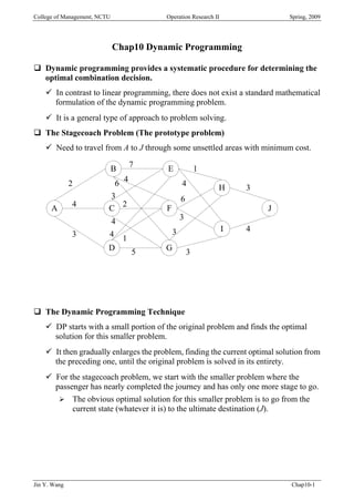
The Stagecoach Problem (The prototype problem)
Need to travel from A to J through some unsettled areas with minimum cost.

B 7 E 1
2 6 4 4 H 3
3 6
A 4 C 2 F J
4 3
3 I 4
3 4 1
D 5 G 3

The Dynamic Programming Technique
DP starts with a small portion of the original problem and finds the optimal
solution for this smaller problem.
It then gradually enlarges the problem, finding the current optimal solution from
the preceding one, until the original problem is solved in its entirety.
For the stagecoach problem, we start with the smaller problem where the
passenger has nearly completed the journey and has only one more stage to go.
The obvious optimal solution for this smaller problem is to go from the
current state (whatever it is) to the ultimate destination (J).

Jin Y. Wang Chap10-1


At each subsequent iteration, the problem is enlarged by increasing by 1 the
number of stages left to go to complete the journey.
For this enlarged problem, the optimal solution for where to go next from
each possible state can be found relatively easily from the results obtained
at the preceding iteration.

Using DP to solve the stagecoach problem
Decision variables: xn (n = 1, 2, 3, 4) denotes the immediate destination on stage
n. That is, the route is A x1 x2 x3 x4, where x4 is J.
Let fn(s, xn) be the total cost of the best overall policy for the remaining stages,
given that the passenger is in state s, ready to start stage n, and selects xn as the
immediate destination.

Given s and n, let xn* denote any value of xn (not necessary unique) that
minimizes fn(s, xn), and let fn*(s) be the corresponding minimum value of
fn(s, xn).

Thus, fn*(s) = min f n ( s, x n ) = fn(s, xn*), where fn(s, xn) = c sx + f n*+1 ( x n ) .
x n
n

Because the ultimate destination (J) is reached at the end of stage 4, f5*(J) = 0.
The objective is to find f1* (A) and the corresponding routes.



Solution procedure for the prototype problem
n = 4. When the passenger has only one more stage to go (n = 4), his route
thereafter is determined entirely by this current state s (either H or I) and his
final destination x4 = J, so the route for this final stagecoach run is s J.
s (current state) f4*(s) x4*
H
I

H 3

J

I 4

n = 3,
s (current state) f 3 ( s, x3 ) = c sx3 + f 4* ( x3 ) f3*(s) x3*
H I
E
F
G

n = 2,
s (current f 2 ( s, x 2 ) = c cx2 + f 3* ( x 2 ) f2*(s) x2*
state) E F G
B
C
D



n = 1,
f1 ( s, x1 ) = ccx1 + f 2* ( x1 ) f1*(s) x1*
B C D
A
An optimal solution for the entire problem can be identified from these four
tables.

B 7 E 1
2 6 4 4 H 3
3 6
A 4 C 2 F J
4 3
3 I 4
3 4 1
D 5 G 3

Characteristics of Dynamic Programming Problems
The problem can be divided into stages, with a policy decision required at each
stage.
In the stagecoach problem, there are four stages.
The policy decision at each stage was which next destination to choose.
Each stage has a number of states associated with the beginning of that stage.
The states are the various possible conditions in which the system might be
at that stage of the problem.



The number of states may be either finite or infinite.
The effect of the policy decision at each stage is to transform the current state to
a state of the next stage.
The solution procedure is designed to find an optimal policy for the overall
problem, i.e., a prescription of the optimal policy decision at each stage for each
of the possible states.
In addition to identifying three optimal solutions (in our prototype
problem), the results show the passenger how he should proceed if he gets
detoured to a state that is not on an optimal route.
Given the current state, an optimal policy for the remaining stages is
independent of the policy decisions adopted in previous stages.
The optimal immediate decision depends on only the current state and not
on how you get there. This is the principle of optimality for DP.
The solution procedure begins by finding the optimal policy for the last stage.
A recursive relationship that identifies the optimal policy for stage n, given the
optimal policy for stage n+1 is available.
In the stagecoach problem, f n* ( s ) = min x {c sx + f n*+1 ( x n )}.
n n

Summary of notations used.
N = number of stages.
n = label for current stage (n = 1, 2, …, N).
sn = current state for stage n.
xn = decision variable for stage n.
xn* = optimal value of xn.
fn(sn, xn) = contribution of stages n, n+1,…, N to objective function if
system starts in state sn at stage n, immediate decision is xn, and optimal
decisions are made thereafter.
fn*(sn) = fn( sn, xn* ).
The recursive relationship will always be of the form
fn*(sn) = max{ f n ( s n , x n )} or fn*(sn) = min{ f n ( s n , x n )}
x
xn n

When we use this recursive relationship, the solution procedure starts at the end
and moves backward stage by stage—each time finding the optimal policy for
that stage— until it finds the optimal policy starting at the initial stage.
Deterministic Dynamic Programming
The state and the next stage are completely determined by the state and policy
decision at the current stage.



Distribution Medical Teams to Countries Example
It has five medical teams available to allocate among three countries.
We need to determine how many teams to allocate to each country to maximize
the total effectiveness.
Thousands of Additional Person-Year of Life
Medical Country
Teams 1 2 3
0 0 0 0
1 45 20 50
2 70 45 70
3 90 75 80
4 105 110 100
5 120 150 130
Stages: these three countries can be considered as the three stages.
Decision variables: xn (n = 1, 2, 3) are the number of teams to allocate to stage
(country) n.
States: sn = number of medical teams still available for allocation.



Recursive relationship function:
Let pi(xi) be the measure of performance from allocating xi medical teams
to country i.
f n ( s n , x n ) = p n ( x n ) + f n*+1 ( s n − x n )
fn*(sn) =

n = 3,
s3 f 3* ( s3 ) *
x3
0
1
2
3
4
5
n = 2,
x2 f 2 ( s 2 , x 2 ) = p 2 ( x 2 ) + f 3* ( s 2 − x 2 ) f 2* ( s 2 ) *
x2
s2 0 1 2 3 4 5
0
1
2
3
4
5

n = 1,
x1 f1 ( s1 , x1 ) = p1 ( x1 ) + f 2* ( s1 − x1 ) f1* ( s1 ) *
x1
s1 0 1 2 3 4 5
5
Thus, x1* = , x2* = , x3* =



Example – Distributing Scientists to Research Teams
Three research teams are trying three approaches to solve a problem.
The probability that these teams will not succeed is 0.4, 0.6, and 0.8,
respectively. Thus, the probability that all three teams will fail is (0.4)(0.6)(0.8)
= 0.192.
In order to minimize the probability of failure, two more scientists are added.
Probability of Failure
New Scientists Team
1 2 3
0 0.40 0.60 0.80
1 0.20 0.40 0.50
2 0.15 0.20 0.30
The problem is to determine how to allocate the two additional scientists to
minimize the probability that all three teams will fail.
Stages: stage n (n = 1, 2, 3) corresponds to research team n.
Decision variables: xn (n = 1, 2, 3) are the number of additional scientists
allocated to team n.
States: sn is the number of new scientists still available for allocation.

Recursive relationship function: f n ( s n ) = min {p n ( x n ) ⋅ f n +1 ( s n − x n )}
* *
x n

pi(xi) denotes the probability of failure for team i if it is assigned xi
additional scientists.

n= 3,
s3 f 3* ( s s ) *
x3
0
1
2



n=2
x2 f 2 ( s s , x 2 ) = p 2 ( x 2 ) ⋅ f 3* ( s 2 − x 2 ) f 2* ( s 2 ) *
x2
s2 0 1 2
0
1
2
n=3
x3 f1 ( s1 , x1 ) = p1 ( x1 ) ⋅ f 2* ( s1 − x1 ) f1* ( s1 ) *
x1
s3 0 1 2
2
Optimal solution:
Example – Scheduling Employment Levels
The workload for a company is subject to considerable seasonable fluctuation.
The minimum employment requirement for different seasons.
Season Spring Summer Autumn Winter Spring
Requirements 255 220 240 200 255
Employment will not be permitted to fall below these levels. Any employment
above these levels is wasted at an approximate cost of $2,000 per person per
season.
The hiring and firing costs are such that the total cost of changing the level of
employment from one season to the next is $200 times the square of the
difference in employment levels
Fractional levels of employment are allowed.
Stages
Spring employment level should be 255 obviously (the highest demand).
Stage 1 = summer, Stage 2 = autumn, State 3 = winter, State 4 = spring.
Spring season is the last stage because the optimal value of the decision
variable for each state at the last stage must be either known or obtainable
without considering other stages.
Decision variables: xn = employment level for stage n (n = 1, 2, 3, 4) (x4 = 255)
Let rn = minimum employment requirement for stage n. That is, r1 = 220,
r2 = 240, r3 = 200, and r4 = 255. Thus, rn ≤ xn ≤ 255.
Cost for stage n = 200(xn – xn-1)2 + 2000(xn – rn).



States: states for stage n is sn = xn-1.

Recursive relationship function is
{ }
f n* ( s n ) = min 200 ( x n − s n ) 2 + 2000 ( x n − rn ) + f n*+1 ( x n )
rn ≤ x n ≤ 255

Data summary for this problem
n rn Feasible xn Possible sn = xn-1 Cost
1 220
2 240
3 200
4 255
Stage 4 (n = 4), we already know x4* = 255
s4 f4*(s4) x4*

Stage 3 (n = 3), f 3* ( s 3 ) = 200min255{200 ( x 3 − s 3 ) 2 + 2000 ( x 3 − 200 ) + f 4* ( x 3 )}}
≤x ≤ 3

=
, where 240 ≤ s3 ≤ 255.
How do we determine the optimal value of x3? Recall calculus.
Set the first partial derivative with respect to x3 equal to 0.



Check the second partial derivative.
Check the feasibility of all possible s3.

Substitute x3 into the recursive relationship function

s3 f3*(s3) x3*

Stage 2 (n = 2).
f2* (s2) =

We skip the remaining calculations due to its complexity.
Example – Wyndor Class Company Problem (more than one resource)
Recall the Wyndor problem
Max Z = 3x1 + 5x2
S.T. x1 ≤ 4
2x2 ≤ 12
3x1 + 2x2 ≤ 18
x1, x2 ≥ 0
Stages: these two activities can be interpreted as the two stages.
Decision variables: xn is the decision variable at stage n.
States: sn = amount of respective resources still available.
sn = (R1, R2 , R3), where Ri is the amount of resource i remaining to be allocated.
Therefore, s1 = (4, 12, 18), s2 = (4 – x1, 12, 18 – 3x1)



f2(R1, R2 , R3, x2) = contribution of activity 2 to Z if system starts in state (R1, R2 ,
R3) at stage 2 and decision is x2 = 5x2.
f1(4, 12, 18, x1) = contribution of activity 1 and 2 to Z if system starts in state (4,
12, 18) at stage 1, immediate decision is x1, and then optimal decision is made at
stage 2 = 3x1 + 2 xmax {5x2}
2 ≤12
2 x2 ≤18−3 x1
x2 ≥ 0

max
f2* (R1, R2, R3) = 2 x2 ≤ R2 {5x2}
2 x2 ≤ R3
x2 ≥ 0

f1*(4, 12, 18) = max {3x1 + f2* (4 – x1, f12, 18 – 3x1)
x ≤4
1
3 x1 ≤18
x1 ≥ 0

Stage 2 (n = 2)
(R1, R2 , R3) f2* (R1, R2, R3) x2*

Stage 1 (n = 1)
12 18 − 3 x1
f1*(4, 12, 18) = 0≤ x ≤ 4{3 x1 + 5 min{ ,
max }}
1 2 2
Over the feasible interval 0 ≤ x1 ≤ 4 ,

12 18 − 3x1
so that 3 x1 + 5 min{ , }=
2 2

x1* = 2 is the optimal for both cases.



(R1, R2 , R3) f1* (R1, R2 , R3) x1*

The optimal solution is

Probabilistic Dynamic Programming
The next stage is not completely determined by the state and policy decision at
the current stage. Rather, there is a probability distribution for what the next
state will be.

Example – Determining Reject Allowances
A company has received an order to supply one item with stringent quality
requirement. Thus, this company may produce more than one item to obtain an
item that is acceptable.
The acceptable probability is 0.5.
Production cost is $100 per item. Setup cost is $300. The maximum production
runs is 3. Penalty is $1600.
The objective is to determine the policy regarding the lot size that minimizes the
total expected costs.
Stages: n = production run (n = 1, 2, 3).



Decision variables: xn = lot size for stage n.
States: sn = number of acceptable items still needed (1 or 0) at beginning of stage
n.

fn*(0) =
1 xn * 1 xn *
fn*(1) = xmin f n ( sn , xn ) = x min,...{K ( x n ) + x n + ( ) f n +1 (1) + [1 − ( ) ] f n +1 (0)}
n = 0 ,1,... n = 0 ,1 2 2
1 xn *
= xnmin {K ( x n ) + x n + ( ) f n +1 (1)}
= 0 ,1,... 2

where K(xn) is the setup cost.
f4*(1) =
Stage 3 (n = 3)
x3* f3(1, x3) = K(x3) + x3 + 16 (1/2)x3
s3 0 1 2 3 4 5 f3*(s3) x3*
0
1



Stage 2 (n = 2)
x2* f2(1, x2) = K(x2) + x2 + (1/2)x2f3*(1)
s2 0 1 2 3 4 f2*(s2) x2*
0
1

Stage 1 (n = 1)
x1* f1(1, x1) = K(x1) + x1 + (1/2)x1f2*(1)
s1 0 1 2 3 4 f1*(s1) x1*
1

The optimal solution is:


Orchap10

Recommended

Recommended

More Related Content

What's hot

What's hot (20)

Similar to Orchap10

Similar to Orchap10 (20)

Recently uploaded

Recently uploaded (20)

Orchap10