This document discusses various technical considerations for MRI of the knee. It covers proper positioning and fixation of the knee, acquisition of sagittal and axial images, sequences such as T1-weighted, proton density-weighted, and fast spin echo. It also discusses artifacts that can occur such as magic angle effect, metallic artifacts, and techniques for fat suppression. Ensuring the knee is properly positioned and flexed, acquiring a sufficient number of slices, and being aware of potential artifacts are important for accurate MRI evaluation of the knee.

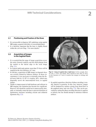
1. 11M. Niitsu et al., Magnetic Resonance Imaging of the Knee,
DOI 10.1007/978-3-642-17893-1_2, © Springer-Verlag Berlin Heidelberg 2013
2.1 Positioning and Fixation of the Knee
It is not possible to diagnose ACL pathology using sagittal•
MR images acquired with fully or overextended knees.
It is therefore important that the knee is slightly flexed•
within the coil (see Chap. 3 for more details).
2.2 Acquisition of Images
in the Sagittal Plane
It is essential that the range of image acquisition covers•
the entire femoral condyles and the tibial plateau from
the medial to the lateral edge in the axial image
(Fig. 2.1).
In a typical adult male patient, more than 25 slices will be•
required at the slice thickness of 3 mm.
In old days, acquisition of MR images in diagonal slices•
was severely limited by foldover artifacts. In those cir-
cumstances, it was necessary to externally rotate the dis-
tal lower limb by 15–20° to visualize ACL, which runs
diagonally across the intercondyloid fossa, in sagittal
images.
Thanks to improvement in both hardware and software in•
MR imaging, this limitation has become less significant.
However, one should be careful not to unnecessarily inter-
nally or externally rotate the knee to prevent distortion of
ligamentous structures including cruciate and collateral
ligaments (Fig. 2.2).
In sagittal acquisition, direction of phase encoding is usu-•
ally anterior to posterior. In this case, however, images
will be hindered by artifacts arising from blood flow in
the popliteal artery and vein (Fig. 2.3). This can be pre-
vented by setting the phase encoding direction to superior
to inferior, but one should attempt to minimize foldover
artifacts.
MRI Technical Considerations
2
Right knee
MedialLateralLateral
Fig. 2.1 Setup of sagittal slices (right knee). In this example, there
are only 17 slices, but ideally, there should be more than 25 slices
at slice thickness of 3 mm to visualize fine changes in cartilage and
menisci

2. 12 2 MRI Technical Considerations
2.3 T1-Weighted and Proton
Density-Weighted Fast Spin-Echo
Sequences
Although both T1- and T2-weighted images are automati-•
cally acquired at many institutions without much consid-
eration, T1-weighted images do not have much value in
delineating ligamentous and meniscal lesions.
Normal ligaments and menisci show low intensity signals,•
and thus proton density- or intermediate-weighted images
will allow better contrast with the surrounding cartilage
and joint fluid (Fig. 2.4).
Fast spin-echo (FSE) sequence requires much shorter•
acquisition time compare to conventional spin-echo (SE)
sequence and enables acquisition of images with higher
anatomical resolution. Thus, FSE is often utilized in knee
MRI.
However, one needs to be cautious regarding the follow-–
ing issues:
Echo train length (ETL) should be kept to the mini-1.
mum to prevent occurrence of blurring of image.
Lateral
Medial
a
b
Fig. 2.2 Example of unsuccessful image acquisition due to excessive
external rotation of the distal lower limb (right knee). Excessive
external rotation of the distal lower limb leads to the direction of sagittal
slice paralleling the lateral wall of intercondyloid fossa (a). In sagittal
images, there will be partial volume effect from the bone cortex, which
also hinders the delineation of ACL (b, arrows)
a
b
Phase encoding direction
Fig. 2.3 Blood flow artifacts arising from inappropriate phase
encoding direction. In sagittal acquisition, direction of phase encoding
is usually anterior to posterior. In this case, however, images will be
hindered by artifacts (a, arrows) arising from blood flow in the popliteal
artery and vein (*). This can be prevented by setting the phase encoding
direction to superior-to-inferior (b)

3. 132.3 T1-Weighted and Proton Density-Weighted Fast Spin-Echo Sequences
a b
c d
Fig. 2.4 Comparison of T1WI and intermediate-weighted (close to
PDW) images. (a) and (c) T1WI (SE 350/14). (b) and (d) intermediate-
weighted (close to PDW) images (FSE 1.324/17, ET 5). The latter
demonstrates the margins of ACL and cartilage better than the T1WI,
also with a better contrast of meniscal tear (d, arrow)

4. 14 2 MRI Technical Considerations
Fat may be depicted as hyperintensity and may lower2.
the contrast against meniscal lesions. This can be pre-
vented by application of fat suppression.
To acquire proton density-weighted FSE images, ETL•
should be kept to the minimum (max 5 or 6).
Using proton density-weighted FSE sequences with•
water-highlighted technique (adding –90° pulse at the
end of the echo train to forcefully recover vertical
magnetization, such as DRIVE (Philips), FRFSE (GE),
RESTORE (Siemens) and T2 Plus (Toshiba)), one can
emphasize the T2-weighted contrast even with a rela-
tive short TR. Joint fluid will be depicted as hyperinten-
sity and with better delineation of cartilage, ligaments,
and menisci (Fig. 2.5).
2.4 Magic Angle Effect
The magic angle effect is a phenomenon that results in•
artifactual hyperintensity in structures with ordered col-
lagen, such as tendons and ligaments. This is because
when collagen is oriented at 55° to the main magnetic
field, dipole-dipole interactions becomes zero, resulting
in a prolongation of T2 relaxation time.
Care must be taken not to mistake this as a pathological•
finding such as a ligamentous tear.
Magic angle effect is particularly notable with short•
TE sequences such as T1-weighted, proton density-
weighted, or T2*-weighted (which is based on a gradient-
recalled echo sequence using a low flip angle) sequences
(Fig. 2.6).
Magic angle effect can also affect the posterior horn of the•
lateral meniscus (Fig. 2.7).
Magic angle effect can be avoided by using a long TE.•
Therefore, if magic angle effect is seen in T2*-weighted
images, it can be eliminated by using SE sequences with
a long TE or T2-weighted FSE sequences (Fig. 2.8).
References
Erickson SJ, et al. The “magic angle effect”: background and clinical
relevance. Radiology. 1993;188:23–5.
Peterfy CT, et al. Magic-angle phenomenon: a case of increased signal
in the normal lateral meniscus on short-TE MR images of the knee.
AJR. 1994;163:149–54.
a b
Fig. 2.5 PDWI with DRIVE (a), in which joint fluid is depicted as
hyperintensity, and conventional PDWI (b). In (a), joint fluid is depicted
as hyperintensity which creates better contrast with cartilage and ACL,
allowing these structures to be more clearly delineated (FOV 150 mm, slice
thickness 3 mm, slice gap 0.3 mm, 23 slices, 512 scan matrix, 864 ZIP, scan
time 6 m)

5. 152.4 Magic Angle Effect
T2-Weighted and T2*-Weighted Images
T2- and T2*-weighted images are useful sequences for
knee imaging because it creates a good contrast between
joint fluid (hyperintensity) and the lesions of ligaments
and menisci. A gradient-recalled echo (T2*-weighted)
sequenceisparticularlyusefulfordelineatingfinelesions.
However, bearing in mind that the magic angle effect can
cause an unwanted artifact, a long TE, SE, or FSE
sequence should be added (either sagittal or coronal).
Bo
55°
Fig. 2.6 Magic angle effect affecting the patellar tendon. T2*WI
(GRE 560/14, flip angle 30°). Superior aspect of the patellar tendon
exhibits localized hyperintensity (arrows). This phenomenon can be
seen when the tendon is oriented at 55° to the main magnetic field
(Bo, superior-inferior direction)
Fig. 2.7 Magic angle effect affecting the posterior horn of the lat-
eral meniscus. Coronal T2*WI. Normal posterior horn of the lateral
meniscus exhibits localized hyperintensity (arrows)
b
a
Fig. 2.8 TE-dependent nature of the magic angle effect. T2*WI
(GRE 560/14, flip angle 30°) (a) and T2WI (FSE 3,000/90) (b).
Localized hyperintensity at the inferior aspect of the patellar tendon
seen in (a, arrows) disappears if TE is made longer (b)

6. 16 2 MRI Technical Considerations
2.5 In-Phase and Out-of-Phase Imaging
In gradient-recalled echo sequences, signals from fat and•
water vary depending on TE.
Resonance frequency of water is higher than that of fat by•
3.5ppm.Thisequatestoabout220Hz(63.9MHz×3.5ppm)
in a 1.5-T system.
Thus, resonance frequencies of water and fat synchronize•
every 4.5 ms of TE (in-phase 220 Hz=4.5 ms).
When out-of-phase, signals from water and fat within the•
same pixel cancel out and the signals are lost. For example,
the boundaries between subcutaneous fat and muscle
or blood vessels will appear black (“boundary effect”)
(Fig. 2.9, Table 2.1).
Multiply these values by 0.5 at 3.0 T, by 1.5 at 1.0 T, and•
by 3 at 0.5 T (Table 2.2)
Note: TE=approx. 14 ms results in in-phase in any case•
2.6 Usefulness of Axial Images
Axial images add useful information to sagittal and coronal•
images, which are mainly used for assessment of ligaments
running in the superior-inferior direction and menisci.
Axial images are particularly suitable for delineation of•
the femoral attachment site of the cruciate ligaments, for
example, partial tear of ACL which can be difficult to
detect in sagittal images
Cross-sectional areas of the hamstrings and patellar ten-•
don, which is used for ACL reconstruction, can be
measured
Medial synovial plica and patellofemoral cartilage (the•
thickest cartilage of the knee joint) are clearly visualized
in axial images and evaluation of patellar subluxation
Fluid collection around menisci, including meniscal cysts,•
can also be clearly visualized
Reference
Roychowdhury S, et al. Using MR imaging to diagnose partial tears of
the anterior cruciate ligament: value of axial images. AJR.
1997;168:1487–91.
2.7 Techniques for Fat Suppression
Lesions that are present within the bone marrow, which•
comprises mostly fatty marrow, and subcutaneous fat
should be assessed using fat suppression techniques.
Chemical shift selective (CHESS) method, Chem Sat•
method=a method which utilizes the difference in reso-
nance frequency between fat and water (224 Hz at 1.5 T)
to add a suppress pulse only to fat signals.
14 15 16 17 18
Fig. 2.9 TE-dependent variability of signal strengths in gradient-
recalled echo sequence (From left, TE=14, 15, 16, 17, and 18 ms).
TE=14 and 18 ms results in in-phase, while out-of-phase images will
be created at TE=approx. 16 ms. When out-of-phase, signals from
water and fat within the same pixel cancel out and the signals are lost.
For example, the boundaries between subcutaneous fat and muscle or
blood vessels will appear black (“boundary effect” (black and white
arrows))
Table 2.1 TE (ms) representing in-phase and out-of-phase at 1.5 T
In-phase 4.5 9.0 13.5 18.0 22.5 27.0
Out-of-phase 2.3 6.8 11.3 15.8 20.3 24.8
Table 2.2 TE (ms) representing in-phase at 1.0 and 1.5 T
In-phase at 1.0 T 6.8 13.5 20.3 27.0
In-phase at 0.5 T 13.5 27.0

7. 172.8 Metallic Artifacts
Short TI (tau) inversion recovery (STIR)=a method based•
on IR technique which sets the TI (tau) to be the null point
for the fat signal.
There is a new method called water selective excita-•
tion. This is an addition of an excitation pulse to the
water, rather than adding a suppression pulse to the fat.
Excitation pulses, which are called binomial pulse (e.g.,
1-1, 1-2-1, 1-3-3-1), are split, and the phase difference
between the resonance frequencies of water and fat is
utilized (Fig. 2.14). Each technique has pros and cons
(Table 2.3).
2.8 Metallic Artifacts
Inevitably, a metallic artifact will arise if there is a ferro-•
magnetic component within the human body.
Staples used in the ACL reconstruction surgery will dis-•
tort the image due to localized magnetic field inhomoge-
neity. In this case, characteristic “signal dropout” in the
direction of frequency encoding and overlapping of the
artifact in a wider range in the phase encoding direction
(Fig. 2.10).
Metallic artifacts are particularly notable with the gradi-•
ent-recalled echo technique, which is sensitive to mag-
netic field inhomogeneity.
Very small metallic particles may be incidentally dis-•
covered at MR imaging (Fig. 2.11). Metallic artifacts
arising from such small objects are localized to a small
area, but one needs to be careful because it can cause a
burn injury.
Table 2.3 Comparison of fat suppression techniques
Technique Pros Cons
CHESS Prolongation of scan time is little, and
there is little limitation in the image
acquisition techniques
Magnetic field inhomogeneity may lead to failure of fat suppression in
an uneven fashion, particularly at the periphery of a large FOV
STIR Homogeneous and almost perfect fat
suppression can be expected
Need for addition of an IR pulse cause a number of restrictions in the
image acquisition technique (especially the need for increased interslice
gap and prolonged scan time)
Selective water excitation Prolongation of scan time is minimal Very sensitive to magnetic field inhomogeneity
Fig. 2.10 Metallic artifact. Status post-ACL reconstruction. (a) Surgical
stables are observed in the femur and tibia in this lateral knee radiograph.
(b) On sagittal PDWI, image distortion due to localized magnetic field
inhomogeneity (arrows) and signal dropout are seen. The phase encoding
direction is superior-inferior, while the frequency encoding direction is
anterior-posterior. (c) Metallic artifacts are particularly notable with the
gradient-recalled echo technique, which is sensitive to magnetic field
inhomogeneity (coronal T2*WI)

8. 18 2 MRI Technical Considerations
ba
Fig. 2.11 Metallic artifact due to a very small metal particle. (a) In
this T2*WI, there is a localized signal dropout and image distortion at
the inferior aspect of the patella (arrows). (b) This was due to a very
small metal particle (arrow) which is just visible on the lateral
radiograph
Fig. 2.10 (continued)
c
phase
freq
b

9. 192.10 Imaging Techniques for Cartilage2.10 Imaging Techniques for Cartilage
2.9 Magnetization Transfer Contrast (MTC)
Method, MT Effect
MRI mostly visualizes protons of free water•
molecules.
Other than free water, there are water molecules that are•
bound to high-molecular-weight proteins, and their reso-
nance frequency ranges a few thousand Hz.
In MTC method, contrast is created by suppression of•
signals from free water by irradiating off-resonance
pulse (i.e., the pulse that is more than a few thousand
Hz away from the resonance frequency of free water
molecules).
MTC method improves the contrast on T2-weighted•
images between joint fluid and hyaline cartilage, which is
mainly composed of collagen and proteoglycan, by
specifically suppressing signals from cartilage (Fig. 2.12).
However, by irradiating MT pulses:
1. Heat will be generated in the body as determined by
the specific absorption rate (SAR)
2. Scan time will be slightly prolonged
FSE techniques that utilize many 180 degree pulses also•
involve the MT effects
2.10 Imaging Techniques for Cartilage
The two most commonly used MR sequences for carti-•
lage imaging are the following (Table 2.4) (Fig. 2.13):
Balanced steady-state free precession (3D balanced•
gradient echo) technique offers a new method to delin-
eate cartilage and includes sequences such as TrueFISP
(Siemens) and Balanced FFE (Philips). Use of a rela-
tively large flip angle leads to depiction of joint fluid as
hyperintensity and enables acquisition of high-contrast
images. Also, TR can be shortened and thus high-quality
cartilage imaging within a short scan time can be
achieved.
Fig. 2.12 Delineation of cartilage using the MTC method. (a)
T2*WI (GRE, 545/15, flip angle 30°) and (b) T2*WI with added MTC
(same parameter as a). In T2*WI, cartilage and joint fluid are both
exhibiting hyperintensity. By addition of MT effect, cartilage signal is
specifically suppressed (arrows) and improves the contrast against
hyperintense joint fluid (arrowhead)
Table 2.4 Comparison of diagnostic performance of T2-weighted FSE
and T1-weighted GRE sequences
Sensitivity for cartilage
defect detection
Specificity for cartilage
defect detection
T2-weighted FSE
with MTC
94% 99%
Fat-suppressed
T1-weighted GRE
75–85% 97%

10. 20 2 MRI Technical Considerations
Fig. 2.14 Delineation of cartilage using 3D balanced gradient-echo
sequence. Balanced FFE (TR/TE=12/6.0, flip angle 70°, 1-3-3-1 selec-
tive water excitation applied, slice thickness 1.6 mm, FOV 140 mm,
matrix 256×512, scan time 4 min 06 s). Joint fluid appears hyperintense,
creating a good contrast against superficial cartilage damage (arrow)
Fig. 2.13 Imaging of hyaline cartilage. In FSE T2WI with MTC (a),
cartilage appears hypointense in contrast to hyperintense joint fluid. In
FS GRE T1WI (b), cartilage appears hyperintense. (a) FSE T2WI with
MTC (TR/TE=38/14, flip angle 30°, off-resonance MTC, scan time
4 min 32 s). (b) FS GRE T1WI (TR/TE=32/6.8, flip angle 25°, fat sup-
pression, scan time 5 min 03 s). Both were 1.5 mm slice thickness,
130 mm FOV, and 256 x 512 matrix
Reference
Disler DG, et al. Fat-suppressed three-dimensional spoiled gradient-echo
MR imaging of hyaline cartilage defects in the knee: comparison with
standard MR imaging and arthroscopy. AJR. 1996;167:127–32.

11. 212.10 Imaging Techniques for Cartilage
Fig. 2.15 3D FS GRE T2*WI of the knee. (a) sagittal (TR/
TE=19/7.0+13.3), (b) coronal reconstruction image, and (c) axial
reconstruction image. (b) and (c) were reconstructed from the sagittal
image (260–320 slices, depending on the size of the knee) to enable
evaluation of cartilage, menisci, synovium, and intra-articular free
bodies
ab
c
a

12. 22 2 MRI Technical Considerations
C B
III
II
I
a
c
b
Fig.2.16 3.0 T MRI of the knee. Coronal image (a) and the magnified
images (b and c). (a) FSE 2,025/20, 3.0/0.3, FOV 160, matrix
1024×1024. (b) Magnified image of the medial compartment shows
three layers of the medial collateral ligament (I, II, III, arrows). The
quality of image is equivalent to that offered by high-resolution images
acquired using microscopy coil (see Chap. 5, Fig. 5.3). (c) Magnified
image of the lateral compartment clearly shows focal cartilage defect of
the lateral femoral condyle (arrow) and distortion of lateral meniscal
free edge (arrow head)

13. 23
Reference
Ramnath RR, et al. Accuracy of 3-T MRI using fast spin-echo tech-
nique to detect meniscal tears of the knee. AJR. 2006;187:221–5.
2.10 Imaging Techniques for Cartilage
Advantages and Disadvantage of 3 T MRI
Improved signal-to-noise ratio:•
High-resolution image: thin slice thickness,–
small FOV, 1024 matrix size
Shorter scan time, increased acquisition series–
Prolongation of T1 values and slight shortening of•
T2 values (but this is not a significant disadvantage
for knee imaging)
Chemical shift becomes more notable (and thus•
adjustment of bandwidth and the use of fat suppres-
sion is required)
Lower RF infiltration, signal inhomogeneity (multi-•
channel, parallel imaging may be needed)
Increased magnetization effect (increased metal-•
related artifact, application to susceptibility imaging)
IncreasedSAR(bewareofexcessiveheatproduction)•
Image Acquisition Protocol for the Most of Images Used
in This Book
1.5 T
Slice thickness 3.0–3.5 mm, slice gap 0.3–0.5 mm
Sagittal images: 23 slices, coronal and axial images:
18 slices
FOV 140–150 mm, matrix 512×256 or 864×512
Intermediate-weighted (close to proton density-•
weighted, and thus in this book, it will be called
“proton density-weighted”) FSE: 1,300–2,500/13–
17, ET 4–6 (+DRIVE if appropriate).
Fat-suppressed proton density-weighted images:•
fat-suppression (e.g., 1-3-3-1 water excitation
pulse) is added to the above sequence.
T2*-weighted image: GRE 500–700/14–15, flip•
angle 25–35°.
T2-weighted images: FSE 2,500–3,500/90–100, ET•
10–15.
T1-weighted images (tumors and bone marrow•
pathologies, only with contrast-enhanced imaging):
SE 350–500/11–17.
3.0 T
2D imaging
Slice thickness 2.0–2.5 mm, slice gap 0.2–0.3 mm
Sagittal images: 26–30 slices, coronal and axial images:
26 slices
FOV 150 mm, matrix 864×512 or 1024×864
Proton density-weighted FSE: 2,400–2,800/17–30,•
ET 4–7 (+DRIVE if appropriate).
Fat-suppressed proton density-weighted images: fat•
suppression (e.g., 1-3-3-1 water excitation pulse) is
added to the above sequence.
T2-weighted and T1-weighted images: almost iden-•
tical to 1.5 T imaging.
3D imaging
Slice thickness 0.6 mm/−0.3 mm (overlapping)
Sagittal images: 280 slices, coronal and axial images:
reconstructed from the sagittal images, FOV 150 mm,
matrix 512×512 (0.3×0.3×0.3 mm isovoxel)
Fat-suppressedT2*-weighted3DGRE:19/7.0+13.3•
(addition of first echo and second echo), fat sup-
pression (e.g., 1-3-3-1 water excitation pulse)
Abbreviations: SE spin echo, FSE fast spin echo, GRE
gradient echo, ET echo train length

14. http://www.springer.com/978-3-642-17892-4