3. A
N
T
H
O
N
Y
I
S
A
A
C
3
7
2
7
B
U
Learning Objectives
Identify dependent and independent variables.■■
Understand variables’ levels of measurement.■■
Explain the differences among nominal, ordinal, interval, and
ratio level data.■■
Determine the level of measurement for variables■■
Now begins the process of statistical analysis. To be able to
4. discuss the charac-
teristics (social phenomena) of our surroundings in terms of
statistics, these charac-
teristics must be in a form suitable for statistical analysis. Like
most mathematical
operations, this is undertaken by organizing the characteristics
in terms of variables.
In “Logic of Comparisons and Analysis” (Chapter 1) you
learned that this process
is called operationalization. Operationalization is the process of
measuring a variable.
This is typically done by assigning numbers to the
characteristics, thereby putting
them in a form that can be analyzed mathematically, a process
often called measure-
ment. This chapter introduces variables as they are used in
statistical analyses. The
process of transforming characteristics into variables is also
discussed. Finally, the
ways in which data and variables can differ are explained.
1 The Variable Defined2-
At its most basic level, a variable is a social phenomenon,
characteristic, or behavior
that a researcher is trying to learn something about. These are
called variables because
they vary between cases. It would be silly to do research on
people or things that did
not vary; we could simply draw a picture and get the same
results. It is how opinions,
characteristics, and other factors differ among people that is the
object of inquiry. For
example, a topic of research might be to examine the difference
in criminal behavior
between males and females. It is the variation in criminal
behavior that may be the
6. 3
7
2
7
B
U
2 Transforming Characteristics into Data: The 2-
Process of Measurement
Measurement is an important part of the process of scientific
inquiry and is a critical
component of statistical analysis. The level of measurement of
data that has been col-
lected is a determining factor in the type of statistical analyses
that can be used. Incor-
rectly identifying the level of measurement of a variable can be
disastrous to research
because statistical analyses that are not appropriate for the data
could mistakenly be
used, which would give erroneous results. Special attention,
then, should be placed on
understanding measurement.
Peter Caws (1959) offers one of the more complete definitions
of measurement:
Measurement is the assignment of particular mathematical
characteristics
to conceptual entities in such a way as to permit (1) an
unambiguous math-
ematical description of every situation involving the entity and
(2) the ar-
rangement of all occurrences of it in a quasi-serial order.
7. Caws goes on to describe this quasi-serial order as establishing
that for any two occur-
rences, they are either equivalent with respect to the
characteristics being studied or
one is greater than the other.
Measurement itself is a way of assigning numbers, or numbered
symbols, to
characteristics (people, social phenomena, etc.) using certain
rules and in such a
way that the relationships between the numbers reflect the
relationships between the
characteristics or variables being studied. For example, in early
biological theory, a
person’s arms were often measured as one characteristic in
determining criminality.
A number could be assigned to each of 10 people (or each
person’s arms) by measur-
ing an arm’s length with a ruler (the number representing arm
length in inches). If
the number assigned to one person was greater than the number
assigned to another
person, the conclusion would be that the first person had longer
arms than the sec-
ond. A further inference from this relationship could be that the
first person might be
more likely to be criminal than the second. In this case, the
relationship among the
numbers used in measurement corresponds to the relationship
among the persons or
their characteristics.
In fields such as physics or engineering, transforming
characteristics into vari-
ables and data is not a problem. A person conducting research
on the space shuttle can
9. 3
7
2
7
B
U
this easy. In many instances, researchers must work to find
ways to turn characteristics
into data. This is sometimes accomplished by classifying the
characteristics into cat-
egories of the variable defined by the researcher. For instance, a
researcher might want
to know whether a person being studied has been convicted of a
crime. When develop-
ing the research methodology for this project, the researcher
could decide there are two
categories of concern: convicted and not convicted. To
transform the characteristics of
the people being studied into data, the categories to be used
might be predefined as 1 to
represent convicted and 0 to represent not convicted. Then,
when the data is gathered,
all that must be done is to code all convicted persons as 1 and
all nonconvicted persons
as 0; thus, the characteristics have been turned into data for the
variable criminal. This
is the process of measurement.2
A distinction should be made here between the measurement
that will be under-
taken in this text and the measurement required when
conducting research. In conduct-
10. ing research, it is important to measure accurately the
phenomena of study, such as
whether the IQ test is a valid measure of intelligence. In fact,
there is a field of study
in measurement theory that addresses the validity of
measurement. In this text the
only requirement is to identify correctly the level of
measurement of data. It will be
assumed that the variables used are a valid measure of the
phenomena being studied.
Sometimes there is also confusion about the difference between
definition and
measurement. Definitions usually replace a word with more
words that simply clarify
meaning. Measurement, on the other hand, assigns a numeric
term that can be ana-
lyzed mathematically or statistically. A definition, then, helps
clarify a concept but
does not require great precision; a definition may be needed for
part of the definition.
Measurement, however, specifies how characteristics will be
grouped on any particu-
lar social phenomenon in a manner that makes it clear what
groups the characteristics
fall into. There may be a few accepted definitions, or there may
be only one (e.g.,
from Webster’s dictionary). Measurement, however, is based on
the research. It is how
you are going to operationalize the concept (as discussed in
Chapter 1 “The Logic of
Comparisons and Analysis”).
As also stated in “The Logic of Comparisons and Analysis,” it
is important to
remember that variables are only representations of the
12. A
N
T
H
O
N
Y
I
S
A
A
C
3
7
2
7
B
U
3 How Variables Can Differ2-
In analyzing variables, it is important to know the ways in
which they differ. Different
types of variables have different characteristics and require
different statistical meth-
ods for proper analysis. Proper classification of a variable is
thus a very important step
in research and in statistical analysis because everything that
follows is dependent on
this proper classification.
Variables can differ in three primary ways. First, they can differ
in their level of
13. measurement. The mathematical characteristics of the variable
crime, discussed above,
are different from the mathematical characteristics of a person’s
attitude toward crime.
Variables can also differ in their scale continuity. Some
variables, such as the number
of children a person has, are whole numbers with no fractions in
between. Other vari-
ables have many values in between any two values. For
example, if asked how old you
are, you would probably respond with a whole number such as
19 years old. If pressed,
though, you would be able to describe your age in terms of
years and months, or years,
months, and days, and so on. Whole numbers represent discrete
variables; while vari-
ables that can be further subdivided represent continuous
variables. Finally, variables
differ in the ways in which they are used in the research
process. Dependent variables
are the object of inquiry: for example, criminal behavior. These
are the characteristics
we want to know something about. Independent variables are
used to describe char-
acteristics of that object: for example, age and its effect on
criminal behavior. A third
use in the research process, confounding variables, has a
bearing on how the first two
types of variables influence each other. Each of the ways
variables differ is discussed
in this section.
Levels of Measurement
The level of measurement is a very important part of classifying
variables for use in
15. D
D
Y
,
A
N
T
H
O
N
Y
I
S
A
A
C
3
7
2
7
B
U
Every variable can be put into one of four categories: nominal,
ordinal, interval,
and ratio. Each of these levels of measurement has different
characteristics that must
be considered when deciding on a statistical procedure.
Nominal Level
16. The lowest level of data in terms of levels of measurement is
nominal level. Nominal
level data is purely qualitative in nature, meaning that the
variables are word ori-
ented, as opposed to quantitative data, which is number
oriented. Variables in this
category might include race, occupation, and hair color. By
assigning numbers to these
characteristics, thereby making them useful for statistical
analysis, we are actually
doing nothing more than renaming them in a numeric format,
and words or letters
would serve just as well. For example, the categories of a
variable could be classified
as either male or female, or these categories could be
abbreviated to M and F. Numbers
could be substituted for these classifications, making them 1
and 2. The numbers are
simply labels or names that can indicate how the groups differ;
but they have no real
numeric significance that can tell magnitudes of differences or
how the numbers are
ordered: male/female, M/F, and 1/2 all mean the same thing
here. Additionally, they
could be switched around such that female/male, F/M, and 2/1
also mean the same
as in the first three instances. The only reason to use numbers
rather than letters is to
make mathematical operations possible.
In operationalizing nominal level data, observations are simply
placed into cat-
egories. The ordering of categories is usually arbitrary. For
example, it makes no dif-
ference when operationalizing eye color whether the brown
category is assigned 0, 1,
17. or 2. The only requirement is that all like scores be coded the
same.
For data to be considered nominal level, the categories of the
variable should be
distinct, mutually exclusive, and completely exhaustive. These
requirements are the
same for ordinal level data.
Distinct means that each value or characteristic of a variable
can be easily sepa-
rated from the other characteristics of that variable. For
example, it is generally easy
to separate male from female participants in a research project.
These categories are
distinct. This task is not always so easy, though. Take, for
example, colors. Depending
on whether you are working from a box of 8 crayons or from a
box of 64, you may
have a difficult time establishing the distinctiveness of, say, the
color red. Also, when
conducting attitudinal surveys, people are seldom totally pro or
con on a subject such
as the death penalty but represent a continuum of attitudes.
Failure to maintain distinc-
tiveness does not characterize the data as being on another level
or as being less than
nominal. It may, however, require that you reconsider or rework
the operationalization
of the variable to ensure it can meet this and other
requirements.
Mutually exclusive means that values fit into only one of the
categories that have
been designated. In the example above, the distinctiveness of
the categories should
19. allow a person to fit into one, and only one, category. In a
study, there should not be
many subjects who can fit into both the male and female
categories. If subjects in a
study can be cross-classified only a few times (as often happens
in any real research
project), it can be dealt with on a case-by-case basis according
to the methodological
plan. Continually finding subjects who can fit into more than
one category, however,
may indicate that you need to reconsider the variable’s
operationalization.
Completely exhaustive means there is a category in which each
characteristic
can be placed. In a research project, there should not be subjects
who do not fit into
one of the categories that were developed. Exhaustiveness is
achieved through careful
planning and operationalization. Researchers must strive to
develop categories that
characterize the variable being studied accurately and
completely. Although “other”
categories are generally effective, they should be used
sparingly. If a large number of
subjects fall into the “other” category, you may need to
reconsider your operationaliza-
tion and create more categories that depict the variable more
accurately. For example,
if the variable race has the categories white, black, and other
but there are a large
number of Latino participants, an additional category may be
necessary.
20. Ordering is the final characteristic of nominal level data. The
primary difference
between nominal level data and other levels of measurement is
that nominal level data
cannot be ordered. Since values are arbitrarily assigned, it
cannot be argued that one
value is greater than or less than another value. For example,
coding blue eyes as 2 and
brown eyes as 1 does not mean that blue eyes are better than
brown eyes. The variable eye
color cannot be ordered in terms of greater or lesser on the
characteristic being studied.
Remember that the most important element of nominal level
data is that the catego-
ries of the data cannot be ordered. The categories being distinct,
mutually exclusive, and
completely exhaustive is important, but violation of these
requirements does not make the
data something less than nominal; it is still nominal level data.
It is very important, then, to
establish the ordering (or lack thereof) of the categories. You
should be very specific as to
why the categories can be ordered or cannot be ordered. Failure
to be very clear concern-
ing the ability to order categories will almost always result in
misclassification of the level
of measurement. For example, you may have data such as patrol
district number, which
you obtained from the local police agency. These patrol district
numbers may appear as
follows:
1
22. 3
7
2
7
B
U
These are certainly ordered, right? Wrong. If you examined
them closely, you
would see that the numbers can be ordered but what they
represent (patrol districts) is
not ordered. You could just as easily have labeled them patrol
districts A, B, C, D, E.
This issue is addressed again later in our discussion of ordinal
level data.
The key in operationalizing and assigning values to nominal
level data is that all
characteristics, sometimes called attributes, that are the same
are assigned the same
value, and characteristics that are different are assigned
different values. To effectively
utilize attributes measured at the nominal level, all values that
are the same should be
coded the same, and very few of the values should have the
possibility of being coded
into more than one category.
As discussed in “Measures of Central Tendency,” “Measures of
Dispersion,”
and “The Form of a Distribution” (Chapters 4, 5, and 6
respectively), most statistical
analyses associated with nominal level data are simple counts
and analyses based on
23. those counts. In these analyses, some assumptions can be made
about how many of
the characteristics are in each category but little else. Since we
are not able to ascribe
true numbers to nominal level data, any procedures requiring a
quantitative measure
generally will not work with those data.
Ordinal Level
Ordinal level data is similar to nominal level data in that it must
also be distinct,
mutually exclusive, and completely exhaustive. Remember,
though, that if an ordinal
level variable is not, for example, distinct, it does not make it
nominal. It is still ordinal
level, but it has some methodological issues of distinctness. The
difference between
nominal and ordinal level data is that ordinal level data can be
ordered.
In ordinal level data, phenomena are assigned numbers; the
order of the numbers
reflects the order of the relationship between the characteristics
being studied. This
order in the categories is such that one may be said to be less
than or greater than
another, but it cannot be said by how much. This ordering is
similar to having a foot
race without a stopwatch: it is possible to determine who
finished first but it is difficult
to determine exactly by how much that runner won. An example
of an ordinal level
variable might be income, where the categories are as follows:
$50,000 and more
25. A
A
C
3
7
2
7
B
U
Values assigned to the categories of ordinal level data may be
expressed either in
words (low, medium, high) or in numbers (1, 2, 3). Either set
may be used as long as
it conveys the ordering of the categories.
There are two different classifications of ordinal level data:
partially ordered and
fully ordered. The differences between them are the number of
data points in the scale
and the degree to which approximate intervals can be
determined.
Partially ordered variables are often expressed in a small
number of categories
(typically less then 5), such as small, medium, and large.
Although it is easy to tell
which has a greater value relative to the other, the magnitude of
differences is impos-
sible to determine. For example, there may be little difference
between a small and a
medium item and a great difference between a medium and a
large item. Here, there
26. are no equal intervals between these categories, precluding them
from rising to interval
level data.
Fully ordered ordinal level data provides more options upon
which to place ranks.
The typical data here is on a scale of 1 to 10. Variables that
have 10 data points instead
of three allow refined measurement and more closely
approximate equal intervals. A
scale of 1 to 100 would allow even greater precision and would
come much closer to
approximating interval level data.
A controversy often arises concerning where partially ordered
data ends and fully
ordered data begins. The issue here is that many people will
attempt to use interval
level analyses with fully ordered ordinal level variables. This is
particularly the case
with Likert scales (discussed later). Although there are no strict
guidelines, general
wisdom on the break between partially ordered and fully
ordered data is that five or
more categories is generally considered fully ordered. Thus, a
scale with five or more
items might be considered fully ordered, whereas a scale with
four items would be
considered partially ordered. Whether it is appropriate to use
interval level analyses
with fully ordered ordinal level data is a more complicated issue
that is addressed
later.
Statistical analyses associated with ordinal level data operate
either from fre-
28. N
T
H
O
N
Y
I
S
A
A
C
3
7
2
7
B
U
nal level data it is not possible to know exactly what the
interval is between, for
example, shirt sizes of small, medium, and large, with interval
level data it is easy to
establish that there are equal intervals between, for example,
miles per gallon in fuel
economy.
Another difference between ordinal and interval level data is the
scale continu-
ity. As discussed later in the section on scale continuity,
interval level data may be
continuous, where there are intermediate values in the scale that
can be divided into
29. subclasses, or discrete, in which there are no values falling
between adjacent values
on the same scale. Ordinal level data is rarely continuous in
nature because, by its
definition, ordinal level data is based on ranks that are
generally represented by whole
numbers (or perhaps gross decimal divisions such as 5.5).
Based on these characteristics, interval level data differs from
ordinal level data
primarily in having equal intervals between values, such as
seconds in a measure of
time, whereas ordinal level data does not, as with a ranking of
fastest to slowest time.
Interval level data is separated from ratio level data, though,
because interval level
data does not have a true zero, which is required for ratio level
data.
Researchers generally want to make variables interval level
because they can then
use interval level statistical analyses, which are more powerful
than ordinal level sta-
tistical analyses. Also, math can be used with interval level data
to draw conclusions
not obvious from the raw numbers.
Special Kinds of Interval Level Data. Since it is desirable to use
interval level
analyses when conducting research, special attempts are often
made to make data
inter val level. Two such instances are using dichotomized data
as interval level and
attempting to make ordinal level scales interval level.
Dichotomized variables are variables that are divided into two
30. categories, such
as male/female and yes/no. Dichotomized variables are
sometimes treated as interval
level. Actually, if the variable represents the presence and
absence of something, it
may be considered ratio. The reason for this is that the two
points can be treated, math-
ematically, the same as other interval level data.3 One of the
identifying characteristics
of interval level data is that it can form a straight line between
points (see Figure 2-1).
The same is true for dichotomized data, with the straight line
running between the two
points. Additionally, because there are only two data points,
there is only one interval;
therefore, there can be no unequal intervals.
As mentioned during the discussion concerning multivariate
analysis, this is the
reason dichotomized variables are often allowed in multivariate
analysis even though
these procedures are normally reserved for interval and ratio
level data. It should be
stressed, however, that even though the interval is equal,
dichotomized variables are
not always normally distributed (see Chapter 4). When sample
sizes are small, there-
fore, interval level statistical analyses may not be appropriate
even though the variable
may be considered as being interval level. Additionally, if there
is a high proportion of
352-3 How Variables Can Differ
16304_CH02_Walker.indd 35 8/3/12 10:59:24 AM
32. (see Chapter 6) for interval level analyses.
Although not necessarily a mathematical question for
dichotomized data, there is
the additional issue of whether the data is actually
dichotomized. As discussed above,
people are rarely either totally pro or totally con on a particular
issue, such as the death
penalty. People typically have a range of emotions, or their
approval or disapproval
depends on the situation. It is possible to force the data into two
categories by making
people choose one or the other, but the reality is that this
attitude is actually repre-
sented as a continuum from pro to con, depending on the
situation. This represents a
special issue for an analysis with dichotomized data. If the
purpose of the research is
not dependent on a true dichotomy, for example, the research is
examining how people
choose rather than what they choose, there is no real problem in
using a dichotomized
variable with an underlying continuum. If the purpose of the
research is to predict
categories, however, the underlying continuum between pro and
con represents a sig-
nificant theoretical problem for the research. Another example
can be drawn from
medicine. If the purpose of the outcome is to study the success
of a surgery based on
whether the person lived or not, the use of dichotomized data is
perfect: 1 = the person
lived; 0 = the person died. If the success is measured in the
quality of the surgery,
however, there is a continuum of success that must be accounted
for; for example, the
34. A
C
3
7
2
7
B
U
type of data should be aware of these problems and be prepared
to consider them in the
theoretical, methodological, and statistical plans of the
research.
The debate surrounding the issue of ordinal level data versus
interval level data inten-
sifies when addressing the use of scales such as Likert4 scales
(1 to 5: strongly disagree,
disagree, neutral, agree, strongly agree) that are used so
frequently in opinion research.
There are actually two issues here. The first is whether a scale
of perhaps five items or
fewer should be considered interval level; the second is whether
any scale should be con-
sidered interval level.
The first issue can be settled more quickly than the second.
Most researchers
agree that any scale based on fewer than five items is difficult if
not impossible to
consider as interval level. Even if there was some argument that
the intervals between
the three or four items were equal, it is unlikely that the data
35. would be sufficiently
normally distributed to allow use of parametric (interval level)
analyses.
The key element in the larger debate is whether a scale can be
considered to have
equal intervals between its items. For example, is the distance
in attitude between strongly
disagree and disagree the same as the distance in attitude
between disagree and neutral?
Although there are equal intervals between 1 and 2 and 4 and 5,
it is much more difficult
to state that there is the same interval between attitudes on this
scale; people simply do
not feel the same about an issue such that this conclusion can be
drawn. There is even
weaker support for this conclusion when the scale includes a
neutral category. Can it be
stated with certainty that the difference between agree and
neutral is the same as between
disagree and neutral, and is that distance the same as between
strongly agree and agree?
It is unlikely.
The reason this debate is important is because the nature of
interval level analyses
is also somewhat in debate. For example, in the strictest sense,
means and standard
deviations, and the statistics based on them, should not be used
with ordinal level data
(see Chapter 4 and beyond). As Stevens (1968) noted, however,
researchers can often
gain a better understanding of the data by using such
procedures, and the procedures
are often robust enough to allow using ordinal level data.
Furthermore, as Abelson and
37. ,
A
N
T
H
O
N
Y
I
S
A
A
C
3
7
2
7
B
U
Ratio Level
Ratio level data is considered the highest order of data. It is
interval level data with
a true zero, where there is the possibility of a true absence of
the characteristic in the
variable. For example, income is generally considered a ratio
level variable. You can
certainly have zero income! This true zero may be implied,
however. For example, sci-
entists have addressed the issue of a true, or absolute, zero in
38. temperature even though
they have never been able to achieve it.
The difference between interval and ratio level data is that
interval level data
has no true zero. For example, ignoring for a moment any
discussions of science or
conception, it is generally accepted that something cannot have
zero age. If something
exists, by definition it should have age, based on how long it
has existed. If this is true,
age has no true zero and is considered interval level instead of
ratio level data.
Another important characteristic of ratio data is that it generally
includes things
that can be counted: dollars, eggs, people, and so on. Under its
definition, if something
can be counted, it should represent whole numbers of the item,
and it is therefore easy
to envision an absence of that item (especially dollars!). This
should not be confused,
however, with the whole numbers that are a part of the ranks in
ordinal level data.
There, no true zero is possible because everything must have a
rank (see Box 2-1).
Even though the ranks are whole numbers, they are not ratio
level.
Box 2-1 A Note About Precision
In this section, you will gain experience in classifying variables
into their levels of
measurement. Often, it will be difficult to obtain a consensus of
whether a variable
is interval or ratio. For example, is the air pressure in a tire
40. R
O
D
D
Y
,
A
N
T
H
O
N
Y
I
S
A
A
C
3
7
2
7
B
U
The presence or absence of a true zero affects the mathematical
procedures that can
be used to analyze the data. Without a true zero, ratios cannot
be employed. If we cannot
use ratios, a particular score cannot be said to be twice (or three
41. times, or four times, etc.)
as much as another. The presence of a true zero allows
researchers to work with the knowl-
edge that the ratios will remain constant even though the
numbers may change (2 is half of
4 and is the same ratio as 12 to 24). In real-world research,
though, interval and ratio are
treated the same. There have been no statistical analyses created
that work with ratio level
data to the exclusion of interval level data, although it is
theoretically possible. Therefore,
data that can be measured at the interval or ratio level is
suitable for higher-order statistical
analyses.
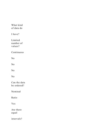
The Process for Determining Level of Measurement
As discussed previously, properly identifying data and
classifying it into its correct
level of measurement is a vital part of the research process. A
practical process for
determining the level of measurement is shown in Figure 2-2.
Using this process will
Can the data be
ordered?
Are there equal
intervals?
Is there a true
zero?
Ratio
Interval
43. O
N
Y
I
S
A
A
C
3
7
2
7
B
U
enable you to examine data (or questions from surveys) and
classify them into the
proper level of measurement.
The first step in this process is to determine if the data can be
ordered. If the data
cannot be ordered, or if the categories can be switched around
such that the ordering
does not matter, the data is considered nominal level. If the data
can be ordered, it is at
least ordinal level and requires further examination.
The next step in this process is to determine if there are equal
intervals between
data points. It should be noted here that equal intervals need not
be present, just the
possibility of equal intervals. For example, when surveying
44. people about their age,
there are definite gaps in the data. This is because there are
usually not enough people
surveyed to have someone at every possible age. This does not
mean the data is not
interval, though, simply because there are not perfect intervals
in the data. If there is no
possibility of equal intervals but the data is ordered, the data is
ordinal. If there is the
possibility of equal intervals between the data points, such as
age in years or months
(where the interval between each data point is 1 year or 1
month, respectively), the
data is at least interval level and requires further examination.
The final step in this process is to determine if there is a true
zero, whether clearly
identifiable or implied. If there is no true zero, the data is
interval; otherwise, the data
is ratio level.
There are a few important points to remember when using this
process to deter-
mine the level of measurement. These will not make the process
of determining the
level of measurement easier, but they will make it more
accurate.
First, it is important to be specific about the data. It is not
enough to think abstractly
about the variable. You have to ask how the data is arranged in
this case. This is partic-
ularly important in establishing whether the data is ordered. It
is not sufficient simply
to state that the data can be ordered. How can it be ordered?
What specifically supports
46. R
O
D
D
Y
,
A
N
T
H
O
N
Y
I
S
A
A
C
3
7
2
7
B
U
interval will probably be different. For example, the difference
between a 5 and a 6 may
be quite different than between a 1 and a 2, because when you
move from a 5 to a 6, you
are saying that the doughnut tastes good rather than just okay,
47. so the interval that may
take a doughnut from a 5 to a 6 is probably larger than to get
from a 1 to a 2. The jump
to get from a 9 to a perfect 10 may be the largest of all because
it takes a great doughnut
to be perfect. The bottom line here is that the intervals between
different categories of
taste are not the same, even though the difference in numbers is
1.
Finally, it is imperative to work through the process outlined in
Figure 2-2 until a
“no” answer is reached. Ordering must be shown for a variable
before equal intervals
matter. There are many variables that have a true zero but
cannot be ordered. Having a
true zero does not matter if the data cannot be ordered; it is still
nominal level data. To
state that a variable is measured at the ratio level, it is
necessary to show all of the fol-
lowing:
The data can be ordered.1.
There are equal intervals.2.
There is a true zero.3.
Also, do not succumb to the temptation to find that a variable
can be ordered and
then quit, stating that it is ordinal. Find out first if there are
equal intervals. If there are
no equal intervals, the variable is ordinal; if there are equal
intervals, the process con-
tinues.
48. Changing Levels
The level of data relies heavily on conceptual grounds, or how
the data is used. For
example, temperature could be measured by those living in the
far north as either
freezing or not freezing, which would be nominal level data.
Others may talk of tem-
perature as either warmer, cooler, or the same, which would be
ordinal level. Gener-
ally, temperature is discussed in terms of degrees Fahrenheit,
which is interval level;
but in science a Kelvin scale is often used, which is ratio level.
In criminological
research, age is generally considered an interval level variable.
If age is being used
simply in its chronological context, it certainly is an interval
level variable. If it is
being used as a measure of maturity, however, not only may it
not be an interval level
variable, but there may be problems supporting age as a valid
measure of maturity (see
the later section on the use of variables in the research process).
As discussed in “The Logic of Comparisons and Analysis”
(Chapter 1), statistical
analysis generally requires the use of analysis procedures
appropriate for the lowest
level of data to be analyzed. For example, if only one variable
in a study is nominal and
the rest are interval, nominal level analyses would be required.
When this occurs, it is
sometimes advantageous to change the level of measurement for
some of the variables.
Most often, this is a process of converting higher levels of data
to lower levels. For
50. example, age, normally interval level, could be converted to
ordinal level by categoriz-
ing it into age groups (0–13 years old, 14–21, 22–30, etc).
Other times, levels of measurement are changed for theoretical
or methodologi-
cal reasons. For example, asking people their exact income does
not always result in
an exact measure because people will guess, and asking the
question in this way may
cause them not to answer the question at all. Allowing
respondents of a survey to
choose an income category rather than write in their income
may obtain a more accu-
rate measure of income, and it may increase the response rate.
Although there are reasons to recode5 variables to lower levels
of measurement,
it should be undertaken with caution and only for proper
reasons. The reason to use
interval and ratio levels of measurement is that it allows
increased precision in the
data. For example, there is less variation between data points in
interval level data,
and the equal intervals allow more precise estimations than do
the unequal intervals
of ordinal level data. On the other hand, it is sometimes
necessary to recode a variable
to get enough data to conduct any analysis at all. As discussed
in “The Form of a Dis-
tribution” (Chapter 6), there are certain requirements for some
statistical analyses that
deal with the size of the groups being studied. Meeting this size
51. requirement some-
times obligates a researcher to recode a variable to obtain a
sufficiently large group.
Typically, this involves combining higher order (interval level)
data into a smaller
number of categories.
Combining different levels of data raises another issue: When
interval level data
is categorized, is it still interval level or is it reduced to ordinal
level? A general rule
is that it is considered ordinal level because it is grouped into
broader categories,
often without equal intervals. In the example above, age
probably would be considered
ordinal because of the categorization and the unequal intervals.
Even if there were
equal intervals, the data would probably still be considered
ordinal level because it is
grouped into a few categories where it is more difficult to
examine the true interval
level relationship between the categories.
It is sometimes possible to change the data from lower to higher
levels of analysis,
but this should be approached cautiously and with a full
understanding of the process.
The researcher must be clear that such changes are not precise
but only approximations.
For example, the most common method of changing to a higher
level of measurement
is through correspondence analysis. Using this statistical
procedure, data that is at the
nominal or ordinal level can be analyzed at the interval level
with certain assump-
tions and limitations. Dichotomizing a variable is another
53. A
A
C
3
7
2
7
B
U
carefully because the overall procedure still violates the
mathematical assumptions of
interval level data.
The bottom line is that all data collection and research is an
exercise in making
trade-offs, and it is sometimes necessary to trade off the level
of measurement to meet
other methodological requirements. The best approach to take is
to gather the data
at the highest level. If the analysis or methodology then
requires categorization that
reduces the level of measurement, this can be done while
retaining the data at a higher
level for other analyses.
Scale Continuity
In addition to their level of measurement, variables can also be
divided into continuous
and discrete scales of measurement. Although not as vital to the
selection and inter-
pretation of statistical analyses as level of measurement, scale
54. continuity is another
method of classifying data, and is used in later discussions. At
this point, only a brief
discussion of the difference between discrete and continuous
data is necessary.
Data is discrete if there are a limited number of values for a
variable. For discrete
variables, only integers (not fractions or decimals) are needed
to label the categories.
For example, the number of crimes committed is generally
represented by integers: 1,
2, 3, and so on.
Continuous variables can have an infinite number of fractions
between them. Age
is a good example of a continuous variable. Depending on how
fine the scale is set, for
example, down to the minutes rather than years, it is not
unlikely that 1000 different
ages could be obtained from 1000 people in a survey. If one
person is 20 years old
and another person is 30, there are many ages that can fit
between these two. Even if
there are two people who are both 20 years old, one born in
January and one born in
December, there are still many people who have different ages
between them. Even
with two people born on the same day, there is the opportunity
for others to be born
between them by measuring the hours or minutes of the time of
birth. As shown in
this example, continuous data can be represented by a large
number of values for any
given variable. Some statistical procedures do not work well or
are difficult to perform
56. H
O
N
Y
I
S
A
A
C
3
7
2
7
B
U
One final note about scale continuity. Be careful about
identifying scale continu-
ity. It is identified as the way the variable is currently being
measured, not its possible
measurement. For example, age can be discrete if it is
categorized either in the data
collection or in the analysis. Again, not that it will detract from
the analysis, but proper
recognition of the scale continuity is important in some
decisions of which statistical
analysis to use.
Use in the Research Process
The final way variables may be classified is by their use in the
research process. Vari-
57. ables may operate in one of three ways in the research process:
as a dependent vari-
able, as an independent variable, or as a confounding variable.
Dependent Variable
In the research process, a dependent variable is one that is the
focus of the research.
Crime is the archetypical dependent variable in criminology and
criminal justice
research, although many others are possible. Dependent
variables are thought to be
influenced by other variables to behave in a certain way. For
example, it is believed
by many that the behavior of a person can be influenced through
learning the behav-
ior from his or her peers. In this type of research, the scores on
the variable criminal
behavior should vary as scores change on the independent
variable(s), which might
include frequency of contact and duration of contact.
It can be difficult to determine the dependent variable,
especially when someone
else’s research is being examined. It is sometimes helpful to see
the dependent variable
as your response if someone asked the topic of your research (or
a term paper). You
would probably respond to the question with something like
“search and seizure” or
“religion in prison.” These, or the variables associated with
these responses, are the
dependent variables for that research.
Independent Variable
59. A
N
T
H
O
N
Y
I
S
A
A
C
3
7
2
7
B
U
An important issue that often gets overlooked in discussing
independent variables
is what actually constitutes an independent variable. It is
common to see variables,
often demographic variables such as age, sex, race, and others,
included in research.
Sometimes these are identified specifically as independent
variables and actually are
used that way in the research process. Sometimes these
variables are called control
variables.6 Used thoughtfully and properly, these demographic
variables are appropri-
ate for research. Often, though, these variables are just
60. “dumped” into the research
with little thought, planning, or discussion. Take the variable
age, for example. Many
criminological studies include age as a variable. Indeed, there is
a strong and sustained
relationship between age and crime that has been supported by
numerous studies. But
is age really an independent variable? The answer is no. Why
would researchers be
interested in the elapsed time since birth? The reason is that age
is actually a proxy for
or an indicator of a more theoretically supportable variable,
maturity. At least theoreti-
cally, an independent variable should be the cause of something
in the dependent vari-
able. The question to ask, then, is: Can age itself cause anything
at all? The answer is,
typically, no; age is more likely to be a proxy, and usually an
imperfect proxy (some
people never grow up), for something else, such as maturity,
that should be included
in the research. Using age as a proxy for a theoretically
supportable variable often
leads to imperfect measures; people will lie about their age and
round off the years
differently. This typically leads to an underestimation of the
real variable. The point
here is that many of the demographic variables included in
research have no real place
as a variable. If the researcher is careful to determine why a
variable such as age is
important to the research, he or she may be able to determine a
more appropriate inde-
pendent variable. That is the variable that should be used.
Confounding Variable
63. officers. Here, the variable duty position is intervening between
education and use of
deadly force. The relationship between these variables is shown
in Figure 2-3.
Spurious variables are similar to intervening variables in that
they detract from the
true relationship between independent and dependent variables,
but spurious variables
operate a bit differently. Spurious variables show a relationship
because of a similar
trend in both variables over time. They influence both the
dependent and independent
variables such that the relationship between the independent and
dependent variables is
inflated. For example, in a research project examining poverty
and crime, there are often
very high correlations between income level and criminality. It
is plausible, though, that
it is not the mere lack of money that is causing the criminality.
It is more likely that the
poverty status of a person is one of many factors, such as where
the person may live,
opportunities, or discrimination, that may be causing the
variation in the dependent vari-
able. Each of these other factors are spurious variables. They
are highly correlated with
poverty status and highly correlated with crime; therefore, they
inflate the relationship
between the two. This relationship is shown in Figure 2-4.
College
Education
Use of Deadly
Force
64. Duty
Position
Independent Variable Dependent VariableIntervening Variable
Figure 2-3 Intervening Variables
Opportunity
Poverty
Status
Criminality
Area of
Residence
Spurious
Variable
Independent
Variable
Dependent
Variable
Spurious
Variable
Figure 2-4 Spurious Variables
46 Chapter 2 n Variables and Measurement
16304_CH02_Walker.indd 46 8/3/12 10:59:25 AM
66. stated above, interven-
ing variables are sometimes included in the theoretical model.
For example, in Figure
2-3, duty position is an intervening variable, but it could have
been included in a
theoretical model shown. Spurious variables, however, are
almost never included
in the theoretical model, or are included erroneously. For
example, it can be argued
that there is a relationship between the salaries of university
professors and the price
of Cuban cigars. Do university professors smoke so many Cuban
cigars that their
economic well-being drives that market? Of course not. Both of
these variables are
influenced by a third, spurious, variable: general increases in
prices and earnings over
time. Since both variables follow the same trends, they appear
to be related, but they
are not.
A final note about variable types: a particular variable can be a
dependent variable
in one study, an independent variable in another, an intervening
variable in another,
and a spurious variable in still another. For example, the
education level of a correc-
tional officer may be a dependent variable in studying the
influence of management
attitudes on increased education; an independent variable, such
as education effects on
inmate abuse; or as a confounding variable such as that between
age and employment
performance. You must be careful, therefore, about how you
look at variables and
make sure of the true role of a variable in a given study.
69. dependent variable ordinal level data
dichotomized variable parametric
discrete variable partially ordered variable
distinct qualitative
fully ordered variable quantitative
independent variable ratio level data
interval level data robust
intervening variable scale continuity
level of measurement spurious variable
measurement true zero
mutually exclusive variation
6 Exercises2-
For each of the variables below: (a) discuss why it is distinct,
mutually exclusive, and
completely exhaustive or why it is not; (b) discuss whether the
variable is discrete or
continuous; (c) work through the process of determining the
level of measurement,
making sure to explain each step; (d) write the level of
measurement for that variable
based on your arguments; and (e) state how the variable would
likely be used in the
research process.
Variables in Everyday Life
1. paint color (red, blue, etc.)
2. miles per hour
3. weight (in pounds)
4. weight (underweight, appropriate, overweight)
5. shirt/blouse size (small, medium, large)
6. number of crimes committed
7. player’s uniform numbers (00, 15, etc.)
8. signs of the zodiac (Aries, etc.)
9. undergraduate major (sociology, engineering, etc.)
71. 7
2
7
B
U
16. religion (Protestant, Catholic, Jewish, Muslim, etc.)
17. schooling (private or public)
18. grade in class (A, B, C, D, F)
19. schooling by type of diploma (elementary, high school,
college)
20. street address numbers
21. size of car (compact, luxury, SUV, etc.)
22. number of people on a committee
23. type of workers (line or staff)
24. marital status (married or not married)
25. make of car (Chevrolet, Ford, etc.)
Variables from Surveys
26. What is your marital status?
(1) ____ never married
(2) ____ married
(3) ____ divorced
(4) ____ separated
(5) ____ widowed
27. What is the size of your community?
(1) ____ rural (unincorporated areas)
(2) ____ rural community (under 10,000)
(3) ____ small city (10,000–49,999)
(4) ____ medium-sized city (50,000–249,000)
(5) ____ large city (over 250,000)
28. What is your social security number?
____ ___ ____
73. Y
I
S
A
A
C
3
7
2
7
B
U
33. What is your major? _____________________
34. Where do you live?
(1) ___ residence hall
(2) ___ fraternity/sorority house
(3) ___ off-campus
35. What were your scores on the SAT/ACT test?
______________
36. Do you consider yourself:
_____ lower class
_____ lower middle class
_____ middle class
_____ upper middle class
_____ upper class
37. What is your age (in years)?
_______
Variables from Statistical Output
38. JOB: What is your occupation?
74. Value Label
Value
Frequency
Percent
Valid
Percent
Cumulative
Percent
Professional 1 105 30.3 34.9 34.9
Clerical/technical 2 43 12.4 14.3 49.2
Blue collar 3 28 8.1 9.3 58.5
Retired 4 68 19.6 22.6 81.1
Housewife 5 16 4.6 5.3 86.4
Other (part-time) 6 28 8.1 9.3 95.7
Unemployed 7 13 3.7 4.3 100.0
Missing 46 13.3
Total 347 100.0* 100.0*
83. 51 1 .3 .3 99.7
79 1 .3 .3 100.0
Missing 10 2.9
Total 347 100.0 100.0
Note: Not all values may be represented in interval/ratio level
tables.
Other Variables to Ponder
Here are some variables whose level of measurement is often
debated. See if you can
determine the level of measurement and present arguments for
why it should be a dif-
ferent level of measurement.
42. Calendar year
43. Hours in a day
Practical Exercise
44. Select three articles from a research journal in criminal
justice or criminology.
Identify and write down (a) the variables used in the research,
(b) the level of
measurement for each variable, (c) why you chose that level of
measurement,
(d) the scale continuity for each variable, and (e) use of the
variable in the
research process.
7 References2-
Abelson, R. P., & Tukey, J. W. (1963). Efficient conversion of
85. O
N
Y
I
S
A
A
C
3
7
2
7
B
U
8 For Further Reading2-
Behan, F. L., & Behan, R. A. (1954). Football numbers.
American Psychologist, 9,
262.
Duncan, O. D. (1984). Notes on Measurement: Historical and
Critical. New York,
NY: Russell Sage Foundation.
Stevens, S. S. (1946). On the theory of scales of measurement.
Science, 103(2684),
677.
Stevens, S. S. (1951). Mathematics, measurement and
psychophysics. In S. S. Stevens
(ed.), Handbook of Experimental Psychology. Hoboken, NJ:
86. Wiley.
9 Notes2-
1. In the current sense of political correctness, the term gender
is frequently used
as a description of whether a person is male or female.
Biologically, however,
the term sex is more accurate in this respect; whereas gender is
more appropri-
ate in examining masculinity/femininity. Throughout this text,
the term sex
will be used to distinguish whether a research subject is male or
female.
2. Although there is no bright line rule about labeling
dichotomized variables
(which gets 0 and which gets 1, or whether to use 0, 1 or 1, 2),
there are some
advantages to a standardized system. For example, when using
yes/no ques-
tions, it is often advantageous to set yes as 1 and no as 0. This
way, the mean
of the variable will be equal to the proportion (p) of yes
answers in the data
and the variance is p(l 2 p). This is particularly useful when the
characteris-
tic under study is set as 1. For example, if you are looking at
the differences
between male and female sentences in courts, you are really
interested in how
females are treated in relation to males. In this case, females
would be given a
score of 1.
3. For example, monotone and affine transformations are
88. I
S
A
A
C
3
7
2
7
B
U
6. A control variable is a variable “held constant” in an attempt
to clarify a
relationship. For example, we know there is a difference
between males and
females in their criminality. After preliminary analyses, then,
the variable sex
might be used to control for this difference, so the research
would only com-
pare males to males and females to females.
Criminal Justice on the Web
Visit http://criminaljustice.jbpub.com/Stats4e to make full use
of today’s teaching and tech-
nology! Our interactive Companion Website has been designed
to specifically complement
Statistics in Criminology and Criminal Justice: Analysis and
Interpretation, 4th Edition. The
resources available include a Glossary, Flashcards, Crossword
Puzzles, Practice Quizzes,
Web links, and Student Data Sets. Test yourself today!