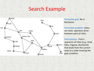
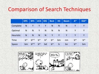
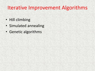
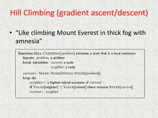
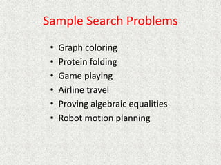
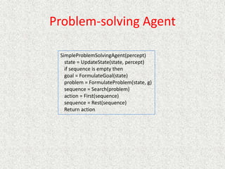
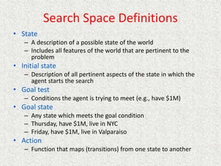
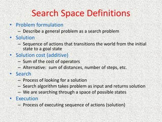
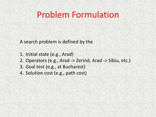
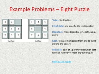
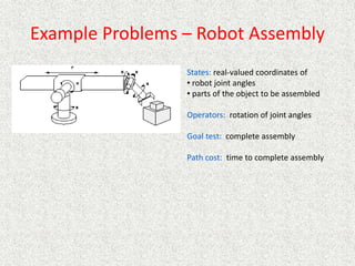
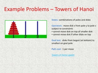
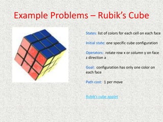
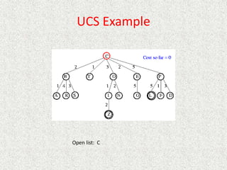
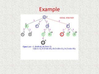
This document discusses search algorithms in artificial intelligence. It describes how search is used to find solutions in many AI problems by exploring possible states. The key aspects covered are: - Search involves exploring a space of possible states through actions or operators to find a goal state. - Problems are formulated as a search problem defined by the initial state, operators/actions, goal test, and cost function. 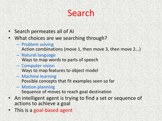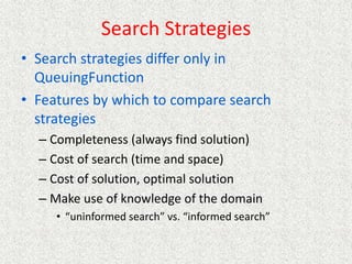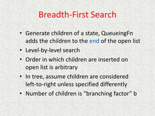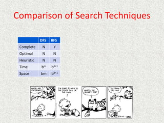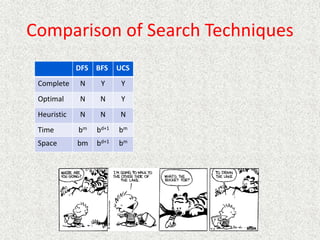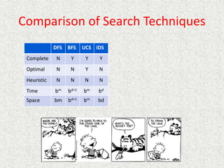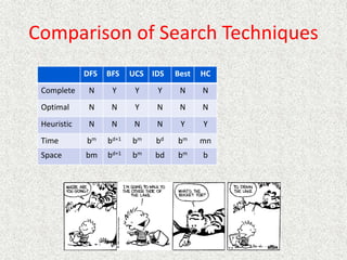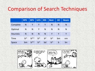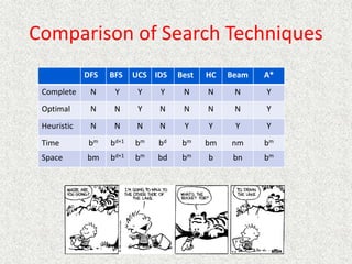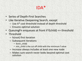- Common uninformed search algorithms like breadth-first search (BFS) and depth-first search (DFS) are described and their properties analyzed. - BFS is complete but can require exponential time and space, while DFS is not complete but uses less space in most cases. 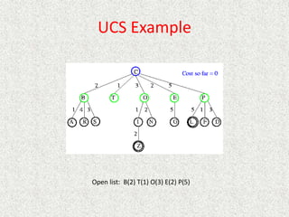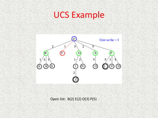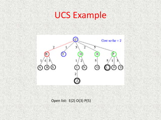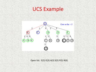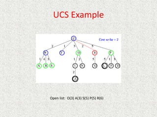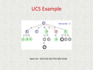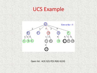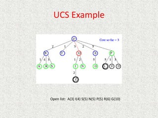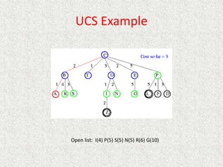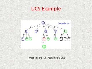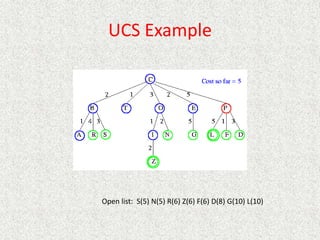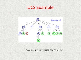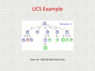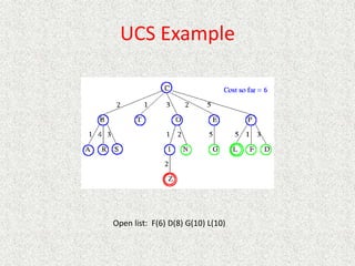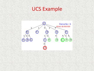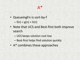- Uniform

1. Artificial Intelligence
Search

2. Search
• Search permeates all of AI
• What choices are we searching through?
– Problem solving
Action combinations (move 1, then move 3, then move 2...)
– Natural language
Ways to map words to parts of speech
– Computer vision
Ways to map features to object model
– Machine learning
Possible concepts that fit examples seen so far
– Motion planning
Sequence of moves to reach goal destination
• An intelligent agent is trying to find a set or sequence of
actions to achieve a goal
• This is a goal-based agent

3. Problem-solving Agent
SimpleProblemSolvingAgent(percept)
state = UpdateState(state, percept)
if sequence is empty then
goal = FormulateGoal(state)
problem = FormulateProblem(state, g)
sequence = Search(problem)
action = First(sequence)
sequence = Rest(sequence)
Return action

4. Assumptions
• Static or dynamic?
Environment is static

5. Assumptions
• Static or dynamic?
• Fully or partially observable?
Environment is fully observable

6. Assumptions
• Static or dynamic?
• Fully or partially observable?
• Discrete or continuous?
Environment is discrete

7. Assumptions
• Static or dynamic?
• Fully or partially observable?
• Discrete or continuous?
• Deterministic or stochastic?
Environment is deterministic

8. Assumptions
• Static or dynamic?
• Fully or partially observable?
• Discrete or continuous?
• Deterministic or stochastic?
• Episodic or sequential?
Environment is sequential

9. Assumptions
• Static or dynamic?
• Fully or partially observable?
• Discrete or continuous?
• Deterministic or stochastic?
• Episodic or sequential?
• Single agent or multiple agent?

10. Assumptions
• Static or dynamic?
• Fully or partially observable?
• Discrete or continuous?
• Deterministic or stochastic?
• Episodic or sequential?
• Single agent or multiple agent?

11. Search Example
Formulate goal: Be in
Bucharest.
Formulate problem: states
are cities, operators drive
between pairs of cities
Find solution: Find a
sequence of cities (e.g., Arad,
Sibiu, Fagaras, Bucharest)
that leads from the current
state to a state meeting the
goal condition

12. Search Space Definitions
• State
– A description of a possible state of the world
– Includes all features of the world that are pertinent to the
problem
• Initial state
– Description of all pertinent aspects of the state in which the
agent starts the search
• Goal test
– Conditions the agent is trying to meet (e.g., have $1M)
• Goal state
– Any state which meets the goal condition
– Thursday, have $1M, live in NYC
– Friday, have $1M, live in Valparaiso
• Action
– Function that maps (transitions) from one state to another

13. Search Space Definitions
• Problem formulation
– Describe a general problem as a search problem
• Solution
– Sequence of actions that transitions the world from the initial
state to a goal state
• Solution cost (additive)
– Sum of the cost of operators
– Alternative: sum of distances, number of steps, etc.
• Search
– Process of looking for a solution
– Search algorithm takes problem as input and returns solution
– We are searching through a space of possible states
• Execution
– Process of executing sequence of actions (solution)

14. Problem Formulation
A search problem is defined by the
1. Initial state (e.g., Arad)
2. Operators (e.g., Arad -> Zerind, Arad -> Sibiu, etc.)
3. Goal test (e.g., at Bucharest)
4. Solution cost (e.g., path cost)

15. Example Problems – Eight Puzzle
States: tile locations
Initial state: one specific tile configuration
Operators: move blank tile left, right, up, or
down
Goal: tiles are numbered from one to eight
around the square
Path cost: cost of 1 per move (solution cost
same as number of most or path length)
Eight puzzle applet

16. Example Problems – Robot Assembly
States: real-valued coordinates of
• robot joint angles
• parts of the object to be assembled
Operators: rotation of joint angles
Goal test: complete assembly
Path cost: time to complete assembly

17. Example Problems – Towers of Hanoi
States: combinations of poles and disks
Operators: move disk x from pole y to pole z
subject to constraints
• cannot move disk on top of smaller disk
• cannot move disk if other disks on top
Goal test: disks from largest (at bottom) to
smallest on goal pole
Path cost: 1 per move
Towers of Hanoi applet

18. Example Problems – Rubik’s Cube
States: list of colors for each cell on each face
Initial state: one specific cube configuration
Operators: rotate row x or column y on face
z direction a
Goal: configuration has only one color on
each face
Path cost: 1 per move
Rubik’s cube applet

19. Example Problems – Eight Queens
States: locations of 8 queens on chess board
Initial state: one specific queens
configuration
Operators: move queen x to row y and
column z
Goal: no queen can attack another (cannot
be in same row, column, or diagonal)
Path cost: 0 per move
Eight queens applet

20. Example Problems –
Missionaries and Cannibals
States: number of missionaries, cannibals,
and boat on near river bank
Initial state: all objects on near river bank
Operators: move boat with x missionaries
and y cannibals to other side of river
• no more cannibals than missionaries on
either river bank or in boat
• boat holds at most m occupants
Goal: all objects on far river bank
Path cost: 1 per river crossing
Missionaries and cannibals applet

21. Example Problems –Water Jug
States: Contents of 4-gallon jug and 3-gallon
jug
Initial state: (0,0)
Operators:
• fill jug x from faucet
• pour contents of jug x in jug y until y full
• dump contents of jug x down drain
Goal: (2,n)
Path cost: 1 per fill
Saving the world, Part I
Saving the world, Part II

22. Sample Search Problems
• Graph coloring
• Protein folding
• Game playing
• Airline travel
• Proving algebraic equalities
• Robot motion planning

23. Visualize Search Space as a Tree
• States are nodes
• Actions are
edges
• Initial state is
root
• Solution is path
from root to
goal node
• Edges
sometimes have
associated costs
• States resulting
from operator
are children

24. Search Problem Example (as a tree)

25. Search Function –
Uninformed Searches
Open = initial state // open list is all generated states
// that have not been “expanded”
While open not empty // one iteration of search algorithm
state = First(open) // current state is first state in open
Pop(open) // remove new current state from open
if Goal(state) // test current state for goal condition
return “succeed” // search is complete
// else expand the current state by
// generating children and
// reorder open list per search strategy
else open = QueueFunction(open, Expand(state))
Return “fail”

26. Search Strategies
• Search strategies differ only in
QueuingFunction
• Features by which to compare search
strategies
– Completeness (always find solution)
– Cost of search (time and space)
– Cost of solution, optimal solution
– Make use of knowledge of the domain
• “uninformed search” vs. “informed search”

27. Breadth-First Search
• Generate children of a state, QueueingFn
adds the children to the end of the open list
• Level-by-level search
• Order in which children are inserted on
open list is arbitrary
• In tree, assume children are considered
left-to-right unless specified differently
• Number of children is “branching factor” b

28. b = 2
Example trees
Search algorithms applet
BFS Examples

29. Analysis
• Assume goal node at level d with constant branching factor b
• Time complexity (measured in #nodes generated)
 1 (1st level ) + b (2nd level) + b2 (3rd level) + … + bd (goal level) + (bd+1 – b)
= O(bd+1)
• This assumes goal on far right of level
• Space complexity
 At most majority of nodes at level d + majority of nodes at level d+1 = O(bd+1)
 Exponential time and space
• Features
 Simple to implement
 Complete
 Finds shortest solution (not necessarily least-cost unless all operators have
equal cost)

30. Analysis
• See what happens with b=10
– expand 10,000 nodes/second
– 1,000 bytes/node
Depth Nodes Time Memory
2 1110 .11 seconds 1 megabyte
4 111,100 11 seconds 106 megabytes
6 107 19 minutes 10 gigabytes
8 109 31 hours 1 terabyte
10 1011 129 days 101 terabytes
12 1013 35 years 10 petabytes
15 1015 3,523 years 1 exabyte

31. Depth-First Search
• QueueingFn adds the children to the
front of the open list
• BFS emulates FIFO queue
• DFS emulates LIFO stack
• Net effect
– Follow leftmost path to bottom, then
backtrack
– Expand deepest node first

32. Example trees
DFS Examples

33. Analysis
• Time complexity
 In the worst case, search entire space
 Goal may be at level d but tree may continue to level m, m>=d
 O(bm)
 Particularly bad if tree is infinitely deep
• Space complexity
 Only need to save one set of children at each level
 1 + b + b + … + b (m levels total) = O(bm)
 For previous example, DFS requires 118kb instead of 10 petabytes for d=12 (10
billion times less)
• Benefits
 May not always find solution
 Solution is not necessarily shortest or least cost
 If many solutions, may find one quickly (quickly moves to depth d)
 Simple to implement
 Space often bigger constraint, so more usable than BFS for large problems

34. Comparison of Search Techniques
DFS BFS
Complete N Y
Optimal N N
Heuristic N N
Time bm bd+1
Space bm bd+1

35. Avoiding Repeated States
• Do not return to parent or grandparent state
– In 8 puzzle, do not move up right after down
• Do not create solution paths with cycles
• Do not generate repeated states (need to store
and check potentially large number of states)
Can we do it?

36. Maze Example
• States are cells in a maze
• Move N, E, S, or W
• What would BFS do
(expand E, then N, W, S)?
• What would DFS do?
• What if order changed to
N, E, S, W and loops are
prevented?

37. Uniform Cost Search (Branch&Bound)
• QueueingFn is SortByCostSoFar
• Cost from root to current node n is g(n)
– Add operator costs along path
• First goal found is least-cost solution
• Space & time can be exponential because large
subtrees with inexpensive steps may be explored
before useful paths with costly steps
• If costs are equal, time and space are O(bd)
– Otherwise, complexity related to cost of optimal
solution

38. UCS Example
Open list: C

39. UCS Example
Open list: B(2) T(1) O(3) E(2) P(5)

40. UCS Example
Open list: T(1) B(2) E(2) O(3) P(5)

41. UCS Example
Open list: B(2) E(2) O(3) P(5)

42. UCS Example
Open list: E(2) O(3) P(5)

43. UCS Example
Open list: E(2) O(3) A(3) S(5) P(5) R(6)

44. UCS Example
Open list: O(3) A(3) S(5) P(5) R(6)

45. UCS Example
Open list: O(3) A(3) S(5) P(5) R(6) G(10)

46. UCS Example
Open list: A(3) S(5) P(5) R(6) G(10)

47. UCS Example
Open list: A(3) I(4) S(5) N(5) P(5) R(6) G(10)

48. UCS Example
Open list: I(4) P(5) S(5) N(5) R(6) G(10)

49. UCS Example
Open list: P(5) S(5) N(5) R(6) Z(6) G(10)

50. UCS Example
Open list: S(5) N(5) R(6) Z(6) F(6) D(8) G(10) L(10)

51. UCS Example
Open list: N(5) R(6) Z(6) F(6) D(8) G(10) L(10)

52. UCS Example
Open list: Z(6) F(6) D(8) G(10) L(10)

53. UCS Example
Open list: F(6) D(8) G(10) L(10)

54. UCS Example

55. Comparison of Search Techniques
DFS BFS UCS
Complete N Y Y
Optimal N N Y
Heuristic N N N
Time bm bd+1 bm
Space bm bd+1 bm

56. Iterative Deepening Search
• DFS with depth bound
• QueuingFn is enqueue at front as with
DFS
– Expand(state) only returns children such that
depth(child) <= threshold
– This prevents search from going down
infinite path
• First threshold is 1
– If do not find solution, increment threshold
and repeat

57. Examples

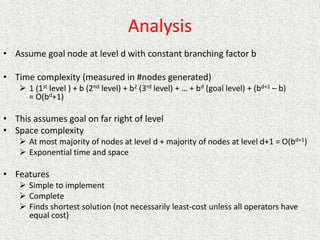
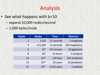
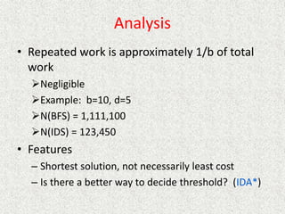
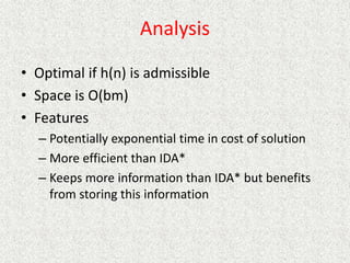
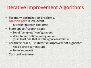
58. Analysis
• What about the repeated work?
• Time complexity (number of generated nodes)
[b] + [b + b2] + .. + [b + b2 + .. + bd]
(d)b + (d-1) b2 + … + (1) bd
O(bd)

59. Analysis
• Repeated work is approximately 1/b of total
work
Negligible
Example: b=10, d=5
N(BFS) = 1,111,100
N(IDS) = 123,450
• Features
– Shortest solution, not necessarily least cost
– Is there a better way to decide threshold? (IDA*)

60. Comparison of Search Techniques
DFS BFS UCS IDS
Complete N Y Y Y
Optimal N N Y N
Heuristic N N N N
Time bm bd+1 bm bd
Space bm bd+1 bm bd

61. Bidirectional Search
• Search forward from initial
state to goal AND
backward from goal state
to initial state
• Can prune many options
• Considerations
– Which goal state(s) to
use
– How determine when
searches overlap
– Which search to use for
each direction
– Here, two BFS searches
• Time and space is O(bd/2)

62. Informed Searches
• Best-first search, Hill climbing, Beam search, A*, IDA*, RBFS, SMA*
• New terms
– Heuristics
– Optimal solution
– Informedness
– Hill climbing problems
– Admissibility
• New parameters
– g(n) = estimated cost from initial state to state n
– h(n) = estimated cost (distance) from state n to closest goal
– h(n) is our heuristic
• Robot path planning, h(n) could be Euclidean distance
• 8 puzzle, h(n) could be #tiles out of place
• Search algorithms which use h(n) to guide search are
heuristic search algorithms

63. Best-First Search
• QueueingFn is sort-by-h
• Best-first search only as good as heuristic
– Example heuristic for 8 puzzle:
Manhattan Distance

64. Example

65. Example

66. Example

67. Example

68. Example

69. Example

70. Example

71. Example

72. Example

73. Comparison of Search Techniques
DFS BFS UCS IDS Best
Complete N Y Y Y N
Optimal N N Y N N
Heuristic N N N N Y
Time bm bd+1 bm bd bm
Space bm bd+1 bm bd bm

74. Hill Climbing (Greedy Search)
• QueueingFn is sort-by-h
– Only keep lowest-h state on open list
• Best-first search is tentative
• Hill climbing is irrevocable
• Features
– Much faster
– Less memory
– Dependent upon h(n)
– If bad h(n), may prune away all goals
– Not complete

75. Example

76. Example

77. Hill Climbing Issues
• Also referred to as gradient descent
• Foothill problem / local maxima / local minima
• Can be solved with random walk or more steps
• Other problems: ridges, plateaus
values
states
local maxima
global maxima

78. Comparison of Search Techniques
DFS BFS UCS IDS Best HC
Complete N Y Y Y N N
Optimal N N Y N N N
Heuristic N N N N Y Y
Time bm bd+1 bm bd bm mn
Space bm bd+1 bm bd bm b

79. Beam Search
• QueueingFn is sort-by-h
– Only keep best (lowest-h) n nodes on open list
• n is the “beam width”
– n = 1, Hill climbing
– n = infinity, Best first search

80. Example

81. Example

82. Example

83. Example

84. Example

85. Example

86. Example

87. Example

88. Example

89. Comparison of Search Techniques
DFS BFS UCS IDS Best HC Beam
Complete N Y Y Y N N N
Optimal N N Y N N N N
Heuristic N N N N Y Y Y
Time bm bd+1 bm bd bm bm nm
Space bm bd+1 bm bd bm b bn

90. A*
• QueueingFn is sort-by-f
– f(n) = g(n) + h(n)
• Note that UCS and Best-first both improve
search
– UCS keeps solution cost low
– Best-first helps find solution quickly
• A* combines these approaches

91. Power of f
• If heuristic function is wrong it either
– overestimates (guesses too high)
– underestimates (guesses too low)
• Overestimating is worse than underestimating
• A* returns optimal solution if h(n) is admissible
– heuristic function is admissible if never overestimates
true cost to nearest goal
– if search finds optimal solution using admissible
heuristic, the search is admissible

92. Overestimating
• Solution cost:
– ABF = 9
– ADI = 8
• Open list:
– A (15) B (9) F (9)
• Missed optimal solution
A (15)
B (6) C (20) D (10)
E (20) F(0) G (12) H (20) I(0)
3
2
3
15 6 20 10 5

93. Example
A* applied to 8 puzzle
A* search applet

94. Example

95. Example

96. Example

97. Example

98. Example

99. Example

100. Example

101. Example

102. Optimality of A*
• Suppose a suboptimal goal G2 is on the open list
• Let n be unexpanded node on smallest-cost path
to optimal goal G1
f(G2) = g(G2) since h(G2) = 0
>= g(G1) since G2 is suboptimal
>= f(n) since h is admissible
Since f(G2) > f(n), A* will never select G2 for expansion

103. Comparison of Search Techniques
DFS BFS UCS IDS Best HC Beam A*
Complete N Y Y Y N N N Y
Optimal N N Y N N N N Y
Heuristic N N N N Y Y Y Y
Time bm bd+1 bm bd bm bm nm bm
Space bm bd+1 bm bd bm b bn bm

104. IDA*
• Series of Depth-First Searches
• Like Iterative Deepening Search, except
– Use A* cost threshold instead of depth threshold
– Ensures optimal solution
• QueuingFn enqueues at front if f(child) <= threshold
• Threshold
– h(root) first iteration
– Subsequent iterations
• f(min_child)
• min_child is the cut off child with the minimum f value
– Increase always includes at least one new node
– Makes sure search never looks beyond optimal cost
solution

105. Example

106. Example

107. Example

108. Example

109. Example

110. Example

111. Example

112. Example

113. Example

114. Example

115. Example

116. Example

117. Example

118. Example

119. Example

120. Example

121. Example

122. Example

123. Example

124. Example

125. Example

126. Example

127. Example

128. Example

129. Example

130. Example

131. Example

132. Example

133. Analysis
• Some redundant search
– Small amount compared to work done on last
iteration
• Dangerous if continuous-valued h(n) values or
if values very close
– If threshold = 21.1 and value is 21.2, probably only
include 1 new node each iteration
• Time complexity is O(bm)
• Space complexity is O(m)

134. Comparison of Search Techniques
DFS BFS UCS IDS Best HC Beam A* IDA*
Complete N Y Y Y N N N Y Y
Optimal N N Y N N N N Y Y
Heuristic N N N N Y Y Y Y Y
Time bm bd+1 bm bd bm bm nm bm bm
Space bm bd+1 bm bd bm b bn bm bm

135. RBFS
• Recursive Best First Search
– Linear space variant of A*
• Perform A* search but discard subtrees when
perform recursion
• Keep track of alternative (next best) subtree
• Expand subtree until f value greater than
bound
• Update f values before (from parent)
and after (from descendant) recursive call

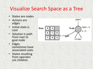
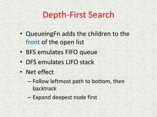
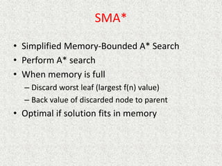
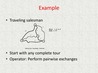
136. Algorithm
// Input is current node and f limit
// Returns goal node or failure, updated limit
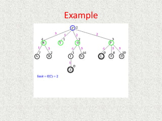
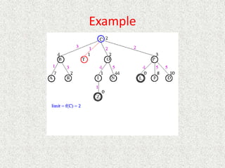
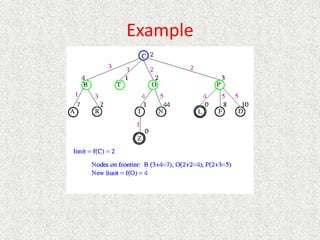
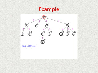
RBFS(n, limit)
if Goal(n)
return n
children = Expand(n)
if children empty
return failure, infinity
for each c in children
f[c] = max(g(c)+h(c), f[n]) // Update f[c] based on parent
repeat
best = child with smallest f value
if f[best] > limit
return failure, f[best]
alternative = second-lowest f-value among children
newlimit = min(limit, alternative)
result, f[best] = RBFS(best, newlimit) // Update f[best] based on descendant
if result not equal to failure
return result

137. Example

138. Example

139. Example

140. Example

141. Example

142. Example

143. Analysis
• Optimal if h(n) is admissible
• Space is O(bm)
• Features
– Potentially exponential time in cost of solution
– More efficient than IDA*
– Keeps more information than IDA* but benefits
from storing this information

144. SMA*
• Simplified Memory-Bounded A* Search
• Perform A* search
• When memory is full
– Discard worst leaf (largest f(n) value)
– Back value of discarded node to parent
• Optimal if solution fits in memory

145. Example
• Let MaxNodes = 3
• Initially B&G added to open
list, then hit max
• B is larger f value so discard
but save f(B)=15 at parent A
– Add H but f(H)=18. Not a
goal and cannot go deper,
so set f(h)=infinity and
save at G.
• Generate next child I with
f(I)=24, bigger child of A.
We have seen all children of
G, so reset f(G)=24.
• Regenerate B and child C.
This is not goal so f(c) reset
to infinity
• Generate second child D
with f(D)=24, backing up
value to ancestors
• D is a goal node, so search
terminates.

146. Heuristic Functions
• Q: Given that we will only use heuristic
functions that do not overestimate, what type
of heuristic functions (among these) perform
best?
• A: Those that produce higher h(n) values.

147. Reasons
• Higher h value means closer to actual distance
• Any node n on open list with
– f(n) < f*(goal)
– will be selected for expansion by A*
• This means if a lot of nodes have a low
underestimate (lower than actual optimum
cost)
– All of them will be expanded
– Results in increased search time and space

148. Informedness
• If h1 and h2 are both admissible and
• For all x, h1(x) > h2(x), then h1 “dominates” h2
– Can also say h1 is “more informed” than h2
• Example
– h1(x):
– h2(x): Euclidean distance
– h2 dominates h1
|
| x
xgoal 
2
2
)
(
)
( y
y
x
x goal
goal 



149. Effect on Search Cost
• If h2(n) >= h1(n) for all n (both are admissible)
– then h2 dominates h1 and is better for search
• Typical search costs
– d=14, IDS expands 3,473,941 nodes
• A* with h1 expands 539 nodes
• A* with h2 expands 113 nodes
– d=24, IDS expands ~54,000,000,000 nodes
• A* with h1 expands 39,135 nodes
• A* with h2 expands 1,641 nodes

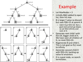
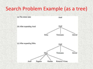
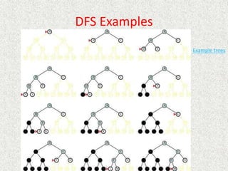
150. Which of these heuristics are admissible?
Which are more informed?
• h1(n) = #tiles in wrong position
• h2(n) = Sum of Manhattan distance between each tile and goal location
for the tile
• h3(n) = 0
• h4(n) = 1
• h5(n) = min(2, h*[n])
• h6(n) = Manhattan distance for blank tile
• h7(n) = max(2, h*[n])

151. Generating Heuristic Functions
• Generate heuristic for simpler (relaxed)
problem
– Relaxed problem has fewer restrictions
– Eight puzzle where multiple tiles can be in the
same spot
– Cost of optimal solution to relaxed problem is an
admissible heuristic for the original problem
• Learn heuristic from experience

152. Iterative Improvement Algorithms
• Hill climbing
• Simulated annealing
• Genetic algorithms

153. Iterative Improvement Algorithms
• For many optimization problems,
solution path is irrelevant
– Just want to reach goal state
• State space / search space
– Set of “complete” configurations
– Want to find optimal configuration
(or at least one that satisfies goal constraints)
• For these cases, use iterative improvement algorithm
– Keep a single current state
– Try to improve it
• Constant memory

154. Example
• Traveling salesman
• Start with any complete tour
• Operator: Perform pairwise exchanges

155. Example
• N-queens
• Put n queens on an n × n board with no two
queens on the same row, column, or diagonal
• Operator: Move queen to reduce #conflicts

156. Hill Climbing (gradient ascent/descent)
• “Like climbing Mount Everest in thick fog with
amnesia”

158. Local Beam Search
• Keep k states instead of 1
• Choose top k of all successors
• Problem
– Many times all k states end up on same local hill
– Choose k successors RANDOMLY
– Bias toward good ones
• Similar to natural selection

159. Simulated Annealing
• Pure hill climbing is not complete, but pure random search
is inefficient.
• Simulated annealing offers a compromise.
• Inspired by annealing process of gradually cooling a liquid
until it changes to a low-energy state.
• Very similar to hill climbing, except include a user-defined
temperature schedule.
• When temperature is “high”, allow some random moves.
• When temperature “cools”, reduce probability of random
move.
• If T is decreased slowly enough, guaranteed to reach best
state.

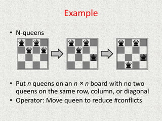
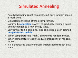
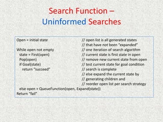
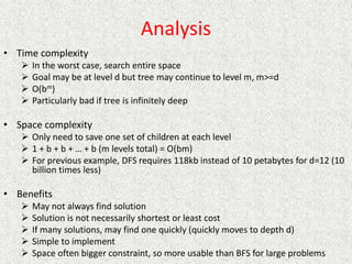
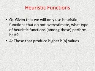
160. Algorithm
function SimulatedAnnealing(problem, schedule) // returns solution state
current = MakeNode(Initial-State(problem))
for t = 1 to infinity
T = schedule[t]
if T = 0
return current
next = randomly-selected child of current
= Value[next] - Value[current]
if > 0
current = next // if better than accept state
else current = next with probability
Simulated annealing applet
Traveling salesman simulated annealing applet
E

E

T
E
e



161. Genetic Algorithms
• What is a Genetic Algorithm (GA)?
– An adaptation procedure based on the mechanics of
natural genetics and natural selection
• Gas have 2 essential components
– Survival of the fittest
– Recombination
• Representation
– Chromosome = string
– Gene = single bit or single subsequence in string,
represents 1 attribute

163. Humans
• DNA made up of 4 nucleic acids (4-bit code)
• 46 chromosomes in humans, each contain 3 billion DNA
• 43 billion combinations of bits
• Can random search find humans?
– Assume only 0.1% genome must be discovered, 3(106) nucleotides
– Assume very short generation, 1 generation/second
– 3.2(10107
) individuals per year, but 101.8(107) alternatives
– 1018106
years to generate human randomly
• Self reproduction, self repair, adaptability are the rule in
natural systems, they hardly exist in the artificial world
• Finding and adopting nature’s approach to computational
design should unlock many doors in science and engineering

164. GAs Exhibit Search
• Each attempt a GA makes towards a solution is
called a chromosome
– A sequence of information that can be interpreted as
a possible solution
• Typically, a chromosome is represented as
sequence of binary digits
– Each digit is a gene
• A GA maintains a collection or population of
chromosomes
– Each chromosome in the population represents a
different guess at the solution

165. The GA Procedure
1. Initialize a population (of solution guesses)
2. Do (once for each generation)
a. Evaluate each chromosome in the population
using a fitness function
b. Apply GA operators to population to create a
new population
3. Finish when solution is reached or number of
generations has reached an allowable
maximum.

166. Common Operators
• Reproduction
• Crossover
• Mutation

167. Reproduction
• Select individuals x according to their fitness
values f(x)
– Like beam search
• Fittest individuals survive (and possibly mate)
for next generation

168. Crossover
• Select two parents
• Select cross site
• Cut and splice pieces of one parent to those of
the other
1 1 1 1 1
0 0 0 0 0
1 1 0 0 0
0 0 1 1 1

169. Mutation
• With small probability, randomly alter 1 bit
• Minor operator
• An insurance policy against lost bits
• Pushes out of local minima
Population:
1 1 0 0 0 0
1 0 1 0 0 0
1 0 0 1 0 0
0 1 0 0 0 0
Goal: 0 1 1 1 1 1
Mutation needed to find the goal

170. Example
• Solution = 0 0 1 0 1 0
• Fitness(x) = #digits that match solution
A) 0 1 0 1 0 1 Score: 1
B) 1 1 1 1 0 1 Score: 1
C) 0 1 1 0 1 1 Score: 3
D) 1 0 1 1 0 0 Score: 3
Recombine top two twice.
Note: 64 possible combinations

171. Example
• Solution = 0 0 1 0 1 0
C) 0 1 1 0 1 1
D) 1 0 1 1 0 0
E) 0 | 0 1 1 0 0 Score: 4
F) 1 | 1 1 0 1 1 Score: 3
G) 0 1 1 0 1 | 0 Score: 4
H) 1 0 1 1 0 | 1 Score: 2
• Next generation:
E) 0 0 1 1 0 0
F) 0 1 1 0 1 0
G) 0 1 1 | 1 0 0 Score: 3
H) 0 0 1 | 0 1 0 Score: 6
I) 0 0 | 1 0 1 0 Score: 6
J) 0 1 | 1 1 0 0 Score: 3
DONE! Got it in 10 guesses.

172. Issues
• How select original population?
• How handle non-binary solution types?
• What should be the size of the population?
• What is the optimal mutation rate?
• How are mates picked for crossover?
• Can any chromosome appear more than once in a
population?
• When should the GA halt?
• Local minima?
• Parallel algorithms?

173. GAs for Mazes

174. GAs for Optimization
• Traveling salesman problem
• Eaters
• Hierarchical GAs for game playing

175. GAs for Control
• Simulator

176. GAs for Graphic Animation
• Simulator
• Evolving Circles
• 3D Animation
• Scientific American Frontiers

177. Biased Roulette Wheel
• For each hypothesis, spin the roulette wheel
to determine the guess

178. Inversion
• Invert selected subsequence
• 1 0 | 1 1 0 | 1 1 -> 1 0 0 1 1 1 1

179. Elitism
• Some of the best chromosomes from previous
generation replace some of the worst
chromosomes from current generation

180. K-point crossover
• Pick k random splice points to crossover parents
• Example
– K = 3
1 1 | 1 1 1 | 1 1 | 1 1 1 1 1 -> 1 1 0 0 0 1 1 0 0 0 0 0
0 0 | 0 0 0 | 0 0 | 0 0 0 0 0 0 0 1 1 1 0 0 1 1 1 1 1

181. Diversity Measure
• Fitness ignores diversity
• As a result, populations tend to become
uniform
• Rank-space method
– Sort population by sum of fitness rank and
diversity rank
– Diversity rank is the result of sorting by the
function 1/d2

182. Classifier Systems
• GAs and load balancing
• SAMUEL