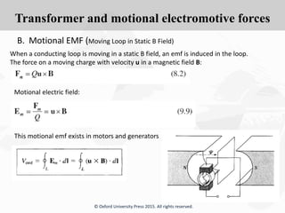
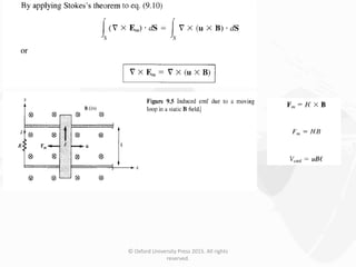
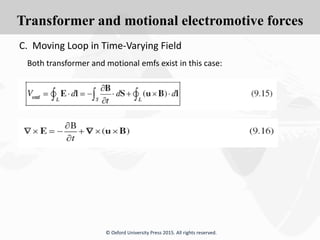
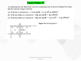
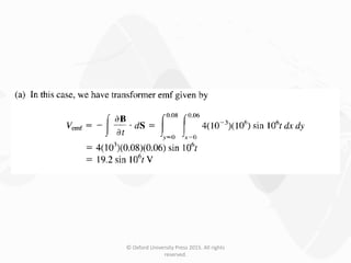
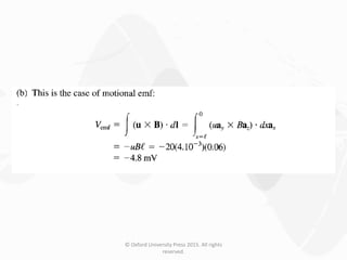
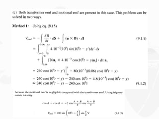
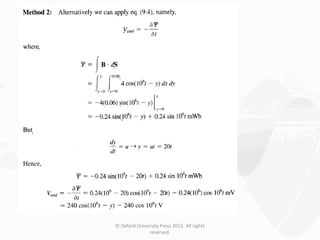
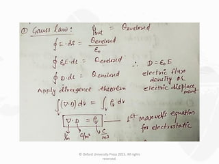
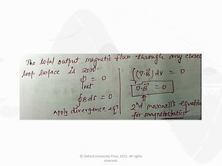
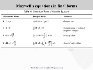
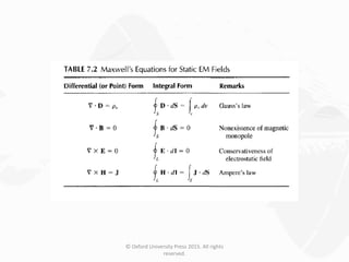
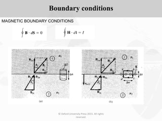
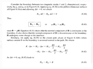
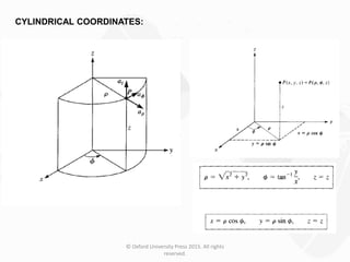
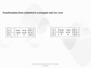
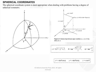
The document discusses Maxwell's equations, which describe the fundamental interactions between electricity and magnetism. It covers topics such as Faraday's law of induction, transformer and motional electromotive forces, displacement current, and Maxwell's equations in their final forms. The document also contains examples of applying Maxwell's equations and discusses boundary conditions at dielectric interfaces.


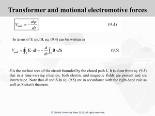


![[Deck] What's New in Spark-Iceberg Integration via DSV2.pptx](https://cdn.slidesharecdn.com/ss_thumbnails/deckwhatsnewinspark-icebergintegrationviadsv2-260210005337-25955b12-thumbnail.jpg?width=640&height=640&fit=bounds)


