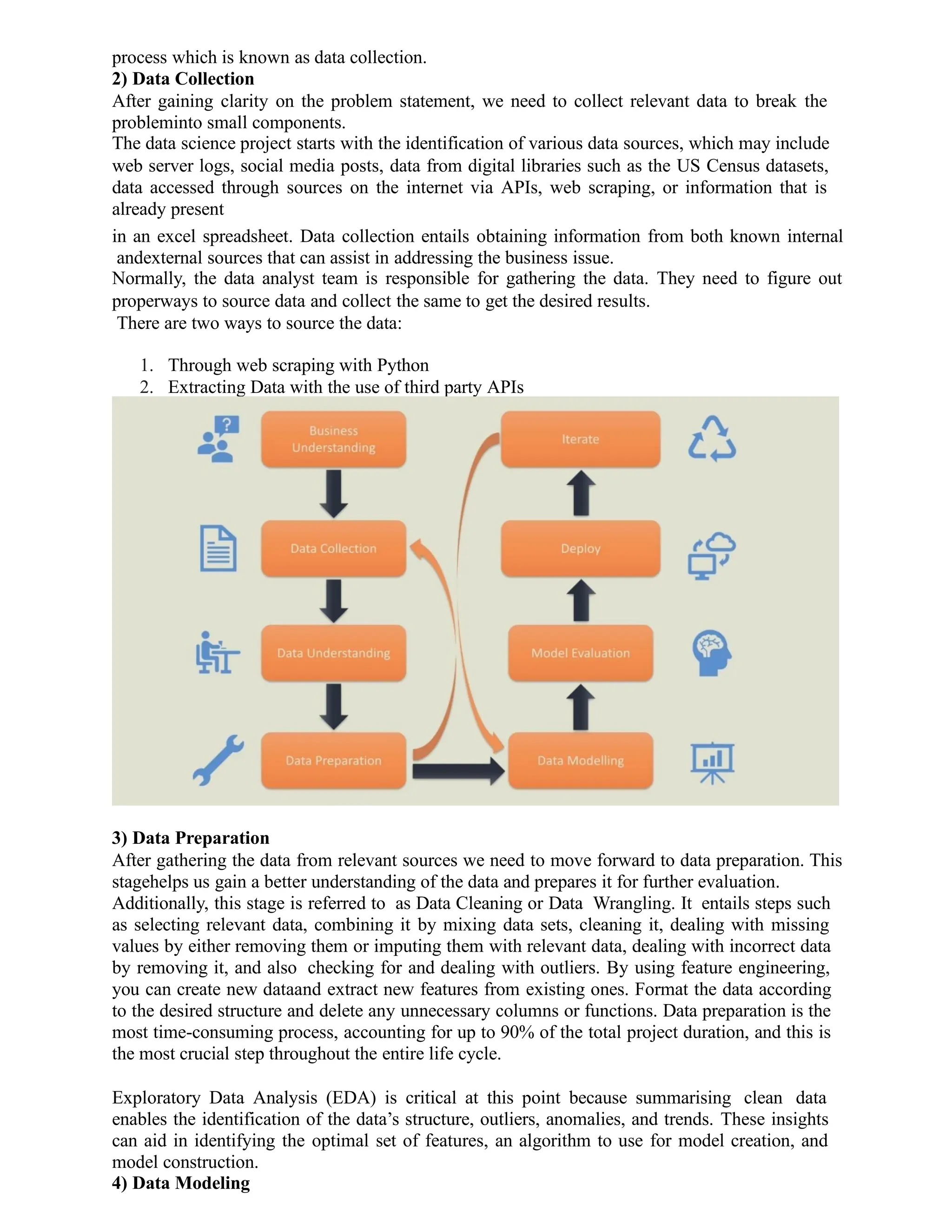
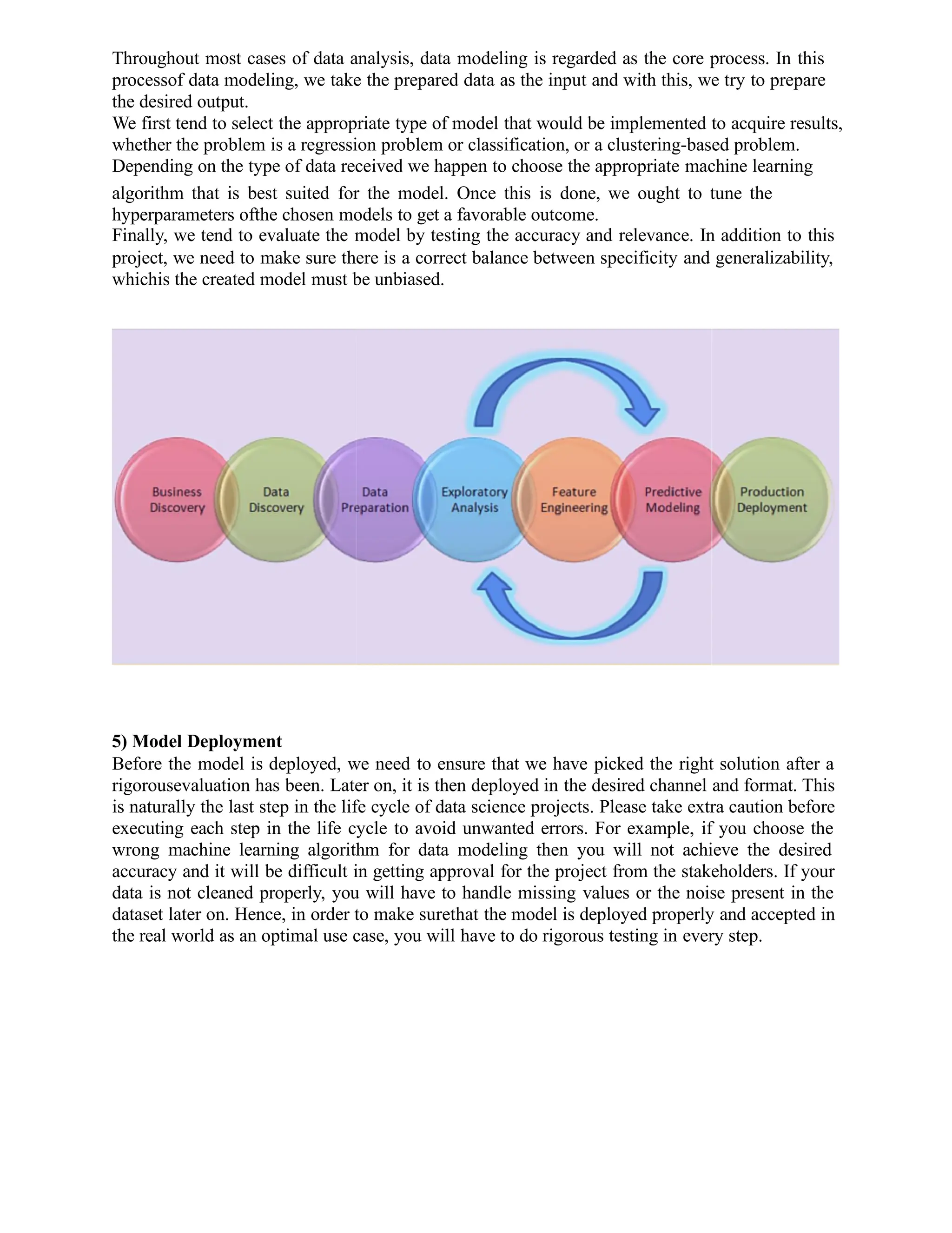
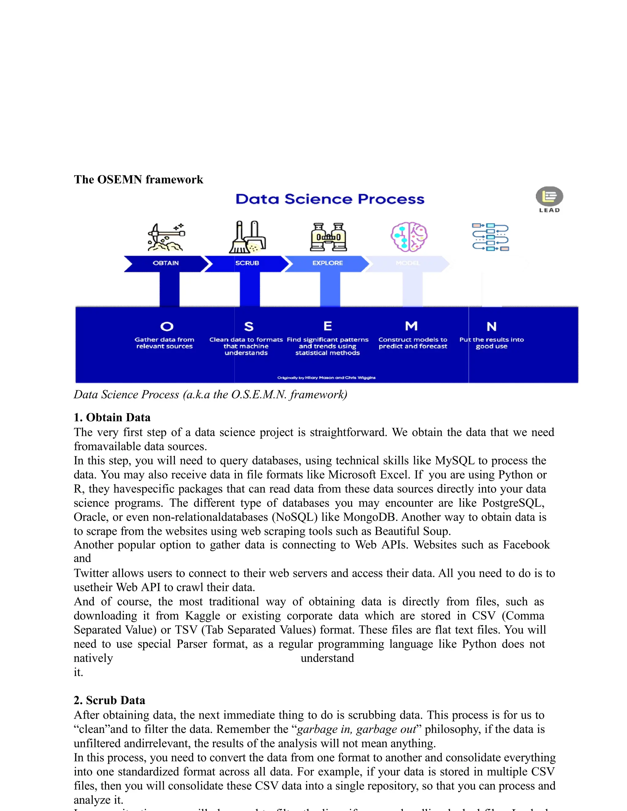
The document outlines the data science project lifecycle, detailing each critical step including understanding the business problem, data collection, data preparation, data modeling, and model deployment. It emphasizes the roles of various team members like business analysts, data analysts, and data scientists in building effective data science projects, as well as the importance of rigorous testing and proper communication of results. Additionally, it introduces the OSEMN framework and highlights essential skills needed in data preprocessing and model interpretation.

1. Data Science Project Lifecycle:
In simple terms, a data science life cycle is nothing but a repetitive set of steps that you need to
take tocomplete and deliver a project/product to your client. Although the data science projects
and the teams involved in deploying and developing the model will be different, every data
science life cycle will be slightly different in every other company. However, most of the data
science projects happen to followa somewhat similar process.
In order to start and complete a data science-based project, we need to understand the
various roles and responsibilities of the people involved in building, developing the project.
Let us take a look atthose employees who are involved in a typical data science project:
Who Are Involved in The Projects:
1. Business Analyst
2. Data Analyst
3. Data Scientists
4. Data Engineer
5. Data Architect
6. Machine Learning Engineer
1) Understanding the Business Problem:
In order to build a successful business model, its very important to first understand the business
problem that the client is facing. Suppose he wants to predict the customer churn rate of his
retail business. You may first want to understand his business, his requirements and what he is
actually wanting to achieve from the prediction. In such cases, it is important to take
consultation from domain experts and finally understand the underlying problems that are
present in the system. A Business Analyst is generally responsible for gathering the required
details from the client and forwarding the data to the data scientist team for further speculation.
Even a minute error in defining the problem and understanding the requirement may be very
crucial for the project hence it is to be done with maximum precision.
After asking the required questions to the company stakeholders or clients, we move to the next

2. process which is known as data collection.
2) Data Collection
After gaining clarity on the problem statement, we need to collect relevant data to break the
probleminto small components.
The data science project starts with the identification of various data sources, which may include
web server logs, social media posts, data from digital libraries such as the US Census datasets,
data accessed through sources on the internet via APIs, web scraping, or information that is
already present
in an excel spreadsheet. Data collection entails obtaining information from both known internal
andexternal sources that can assist in addressing the business issue.
Normally, the data analyst team is responsible for gathering the data. They need to figure out
properways to source data and collect the same to get the desired results.
There are two ways to source the data:
1. Through web scraping with Python
2. Extracting Data with the use of third party APIs
3) Data Preparation
After gathering the data from relevant sources we need to move forward to data preparation. This
stagehelps us gain a better understanding of the data and prepares it for further evaluation.
Additionally, this stage is referred to as Data Cleaning or Data Wrangling. It entails steps such
as selecting relevant data, combining it by mixing data sets, cleaning it, dealing with missing
values by either removing them or imputing them with relevant data, dealing with incorrect data
by removing it, and also checking for and dealing with outliers. By using feature engineering,
you can create new dataand extract new features from existing ones. Format the data according
to the desired structure and delete any unnecessary columns or functions. Data preparation is the
most time-consuming process, accounting for up to 90% of the total project duration, and this is
the most crucial step throughout the entire life cycle.
Exploratory Data Analysis (EDA) is critical at this point because summarising clean data
enables the identification of the data’s structure, outliers, anomalies, and trends. These insights
can aid in identifying the optimal set of features, an algorithm to use for model creation, and
model construction.
4) Data Modeling

3. Throughout most cases of data analysis, data modeling is regarded as the core process. In this
processof data modeling, we take the prepared data as the input and with this, we try to prepare
the desired output.
We first tend to select the appropriate type of model that would be implemented to acquire results,
whether the problem is a regression problem or classification, or a clustering-based problem.
Depending on the type of data received we happen to choose the appropriate machine learning
algorithm that is best suited for the model. Once this is done, we ought to tune the
hyperparameters ofthe chosen models to get a favorable outcome.
Finally, we tend to evaluate the model by testing the accuracy and relevance. In addition to this
project, we need to make sure there is a correct balance between specificity and generalizability,
whichis the created model must be unbiased.
5) Model Deployment
Before the model is deployed, we need to ensure that we have picked the right solution after a
rigorousevaluation has been. Later on, it is then deployed in the desired channel and format. This
is naturally the last step in the life cycle of data science projects. Please take extra caution before
executing each step in the life cycle to avoid unwanted errors. For example, if you choose the
wrong machine learning algorithm for data modeling then you will not achieve the desired
accuracy and it will be difficult in getting approval for the project from the stakeholders. If your
data is not cleaned properly, you will have to handle missing values or the noise present in the
dataset later on. Hence, in order to make surethat the model is deployed properly and accepted in
the real world as an optimal use case, you will have to do rigorous testing in every step.

4. The OSEMN framework
Data Science Process (a.k.a the O.S.E.M.N. framework)
1. Obtain Data
The very first step of a data science project is straightforward. We obtain the data that we need
fromavailable data sources.
In this step, you will need to query databases, using technical skills like MySQL to process the
data. You may also receive data in file formats like Microsoft Excel. If you are using Python or
R, they havespecific packages that can read data from these data sources directly into your data
science programs. The different type of databases you may encounter are like PostgreSQL,
Oracle, or even non-relationaldatabases (NoSQL) like MongoDB. Another way to obtain data is
to scrape from the websites using web scraping tools such as Beautiful Soup.
Another popular option to gather data is connecting to Web APIs. Websites such as Facebook
and
Twitter allows users to connect to their web servers and access their data. All you need to do is to
usetheir Web API to crawl their data.
And of course, the most traditional way of obtaining data is directly from files, such as
downloading it from Kaggle or existing corporate data which are stored in CSV (Comma
Separated Value) or TSV (Tab Separated Values) format. These files are flat text files. You will
need to use special Parser format, as a regular programming language like Python does not
natively understand
it.
2. Scrub Data
After obtaining data, the next immediate thing to do is scrubbing data. This process is for us to
“clean”and to filter the data. Remember the “garbage in, garbage out” philosophy, if the data is
unfiltered andirrelevant, the results of the analysis will not mean anything.
In this process, you need to convert the data from one format to another and consolidate everything
into one standardized format across all data. For example, if your data is stored in multiple CSV
files, then you will consolidate these CSV data into a single repository, so that you can process and
analyze it.

5. files refer to web locked files where you get to understand data such as the demographics of the
users, timeof entrance into your websites etc.
On top of that, scrubbing data also includes the task of extracting and replacing values. If you
realisethere are missing data sets or they could appear to be non-values, this is the time to replace
them accordingly.
Lastly, you will also need to split, merge and extract columns. For example, for the place of
origin, youmay have both “City” and “State”. Depending on your requirements, you might need
to either merge orsplit these data.
Think of this process as organizing and tidying up the data, removing what is no longer needed,
replacing what is missing and standardising the format across all the data collected.
3. Explore Data
Once your data is ready to be used, and right before you jump into AI and Machine Learning,
you willhave to examine the data.
Usually, in a corporate or business environment, your boss will just throw you a set of data and it
is up to you to make sense of it. So it will be up to you to help them figure out the business
question and transform them into a data science question.
To achieve that, we will need to explore the data. First of all, you will need to inspect the data
and
its properties. Different data types like numerical data, categorical data, ordinal and nominal data
etc. require different treatments.
Then, the next step is to compute descriptive statistics to extract features and test significant
variables.Testing significant variables often is done with correlation. For example, exploring the
risk of someonegetting high blood pressure in relations to their height and weight. Do note that
some variables are correlated, but they do not always imply causation.
The term “Feature” used in Machine Learning or Modelling, is the data features that help us to
identify the characteristics that represent the data. For example, “Name”, “Age”, “Gender” are
typical features of members or employees dataset.
Lastly, we will utilise data visualisation to help us to identify significant patterns and trends in
our
data.We can gain a better picture through simple charts like line charts or bar charts to help us to
understandthe importance of the data.
Skills Required
If you are using Python, you will need to know how to use Numpy, Matplotlib, Pandas or Scipy; if
you are using R, you will need to use GGplot2 or the data exploration swiss knife Dplyr. On top of
that, youneed to have knowledge and skills in inferential statistics and data visualization.
As much as you do not need a Masters or Ph.D. to do data science, these technical skills are crucial
inorder to conduct an experimental design, so you are able to reproduce the results.
Additional Tips:
 Be curious. This can help you develop your spidey senses to spot weird patterns and
trends.
 Focus on your audience, and understand their background and lingo. So that you are
able topresent the data in a way that makes sense to them.
4. Model Data
This is the stage where most people consider interesting. As many people call it “where the magic
happens”.

6. Once again, before reaching this stage, bear in mind that the scrubbing and exploring stage are
equally crucial to building useful models. So take your time on those stages instead of jumping
right to this process.
One of the first things you need to do in modelling data is to reduce the dimensionality of your
data set.Not all your features or values are essential to predicting your model. What you need to
do is to selectthe relevant ones that contribute to the prediction of results.
There are a few tasks we can perform in modelling. We can also train models to perform
classification to differentiating the emails you received as “Inbox” and “Spam” using logistic
regressions. We can also forecast values using linear regressions. We can also use modelling to
group data to understand thelogic behind those clusters. For example, we group our e-commerce
customers to understand their behaviour on your website. This requires us to identify groups of
data points with clustering algorithmslike k-means or hierarchical clustering.
In short, we use regression and predictions for forecasting future values, and classification to
identify,and clustering to group values.
5. Interpreting Data
We are at the final and most crucial step of a data science project, interpreting models and data.
The predictive power of a model lies in its ability to generalise. How do we explain a model
depends on itsability to generalise unseen future data.
Interpreting data refers to the presentation of your data to a non-technical layman. We deliver
the results in to answer the business questions we asked when we first started the project,
together with theactionable insights that we found through the data science process.
Actionable insight is a key outcome that we show how data science can bring about predictive
analyticsand later on prescriptive analytics. In which, we learn how to repeat a positive result, or
prevent a negative outcome.
On top of that, you will need to visualise your findings accordingly, keeping it driven by your
business questions. It is essential to present your findings in such a way that is useful to the
organisation, or elseit would be pointless to your stakeholders.
In this process, technical skills only are not sufficient. One essential skill you need is to be able to
tell aclear and actionable story. If your presentation does not trigger actions in your audience, it
means that your communication was not efficient. Remember that you will be presenting to an
audience with no technical background, so the way you communicate the message is key.
Steps involved in data preprocessing
:

7. 1. Importing the required Libraries
2. Importing the data set
3. Handling the Missing Data.
4. Encoding Categorical Data.
5. Splitting the data set into test set and training set.
6. Feature Scaling.
Step 1: Importing the required Libraries
To follow along you will need to download this dataset : Data.csv
Every time we make a new model, we will require to import Numpy and Pandas. Numpy is a
Library which contains Mathematical functions and is used for scientific computing while Pandas is
used to import and manage the data sets.
import pandas as pd
import numpy as np
Here we are importing the pandas and Numpy library and assigning a shortcut “pd” and “np”
respectively.
Step 2: Importing the Dataset
Data sets are available in .csv format. A CSV file stores tabular data in plain text. Each line of the
file is a data record. We use the read_csv method of the pandas library to read a local CSV file as
a dataframe.
1. Reading a CSV file
read_csv
The method of the Pandas library takes a CSV file as a parameter and returns
a dataframe.

8. import pandas as pd
df = pd.read_csv('my_csv.csv')
2. Reading an Excel file
The read_excel method of the Pandas library takes an excel file as a parameter and returns
a dataframe.
import pandas as pd
df = pd.read_excel('my_excel.xlsx')
Once the data has been read into a data frame, display the data frame to see if the data has been
read correctly.
Selecting the dataset:
After carefully inspecting our dataset, we are going to create a matrix of features in our dataset (X)
and create a dependent vector (Y) with their respective observations. To read the columns, we will
use iloc of pandas (used to fix the indexes for selection) which takes two parameters — [row
selection, column selection].
X = dataset.iloc[:, :-1].values
y = dataset.iloc[:, 3].values
Step 3: Handling the Missing Data

9. An example of Missing data and Imputation
The data we get is rarely homogenous. Sometimes data can be missing and it needs to be handled so
that it does not reduce the performance of our machine learning model.
To do this we need to replace the missing data by the Mean or Median of the entire column. For this
we will be using the sklearn.preprocessing Library which contains a class called Imputer which will
help us in taking care of our missing data.
from sklearn.preprocessing import Imputer
imputer = Imputer(missing_values = "NaN", strategy = "mean", axis = 0)
Our object name is imputer. The Imputer class can take parameters like :
1. missing_values : It is the placeholder for the missing values. All occurrences of missing_values
will be imputed. We can give it an integer or “NaN” for it to find missing values.
2. strategy : It is the imputation strategy — If “mean”, then replace missing values using the mean
along the axis (Column). Other strategies include “median” and “most_frequent”.
3. axis : It can be assigned 0 or 1, 0 to impute along columns and 1 to impute along rows.
Now we fit the imputer object to our data.
imputer = imputer.fit(X[:, 1:3])
Now replacing the missing values with the mean of the column by using transform method.

10. X[:, 1:3] = imputer.transform(X[:, 1:3])
Ranking :
Pandas Dataframe.rank() method returns a rank of every respective index of a series passed.
The rank is returned on the basis of position after sorting.
Syntax:
DataFrame.rank(axis=0, method=’average’, numeric_only=None, na_option=’keep’,
ascending=True, pct=False)
Parameters:
axis: 0 or ‘index’ for rows and 1 or ‘columns’ for Column.
method: Takes a string input(‘average’, ‘min’, ‘max’, ‘first’, ‘dense’) which tells pandas what to
do with same values. Default is average which means assign average of ranks to the similar
values.
numeric_only: Takes a boolean value and the rank function works on non-numeric value only if
it’s False.
na_option: Takes 3 string input(‘keep’, ‘top’, ‘bottom’) to set position of Null values if any in the
passed Series.
ascending: Boolean value which ranks in ascending order if True.
pct: Boolean value which ranks percentage wise if True.
# pandas is imported as pd
import pandas as pd
# dictionary is created
data = {'Book_Name':
['Oxford', 'Arihant',
'Pearson', 'Disha',
'Cengage'],
'Author': ['Jhon Pearson', 'Madhumita Pattrea', 'Oscar Wilde', 'Disha', 'G Tewani'],
'Price': [350,880,490,1100,450]}
# creating DataFrame
df = pd.DataFrame(data)
# printing DataFrame
print("Pandas DataFrame:n",df)
print()
# Printing the rank of
DataFrame.
print("Ranking of Pandas
Dataframe:n",df.rank())
Pandas DataFrame:
Book_Name Author Price
0 Oxford Jhon Pearson 350
1 Arihant Madhumita Pattrea 880
2 Pearson Oscar Wilde 490
3 Disha Disha 1100
4 Cengage G Tewani 450
Ranking of Pandas Dataframe:
Book_Name Author Price
0
1
2
3
4
4.0
1.0
5.0
3.0
2.0
3.0 1.0
4.0 4.0
5.0 3.0
1.0 5.0
2.0 2.0
# creating new column Ranked_Author and storing Author column's ranked data in descending order,
df['Ranked_Author']=df['Author'].rank(ascending=False)

11. print("Ranking of Pandas Dataframe Author Column:n",df)
Ranking of Pandas Dataframe Author Column:
Book_Name Author Price
Ranked_Author
0 Oxford Jhon Pearson 350 3.0
1 Arihant Madhumita Pattrea 880 2.0
2 Pearson Oscar Wilde 490 1.0
3 Disha Disha 1100 5.0
4 Cengage G Tewani 450 4.0
Sorting Column with some similar values
import pandas as pd
df = pd.DataFrame.from_dict({
'Date': ['2021-12-01', '2021-12-01',
'2021-12-01', '2021-12-02', '2021-12-
02'],
'Stock_Owner': ['Robert', 'Jhon', 'Maria', 'Juliet', 'Maxx'],
'Stocks': [100, 110, 100, 95, 130]
})
print("Pandas DataFrame:n",df)
print()
df.sort_values("Stocks", inplace = True)
df["Rank"] = df["Stocks"].rank(method ='average')
print("Ranked DataFrame :n",df)
Pandas DataFrame:
Date Stock_Owner Stocks
0 2021-12-01 Robert 100
1 2021-12-01 Jhon 110
2 2021-12-01 Maria 100
3 2021-12-02 Juliet 95
4 2021-12-02 Maxx 130
Ranked DataFrame :
Date Stock_Owner Stocks Rank
3 2021-12-02 Juliet 95 1.0
0 2021-12-01 Robert 100 2.5
2 2021-12-01 Maria 100 2.5
1 2021-12-01 Jhon 110 4.0
4 2021-12-02 Maxx 130 5.0
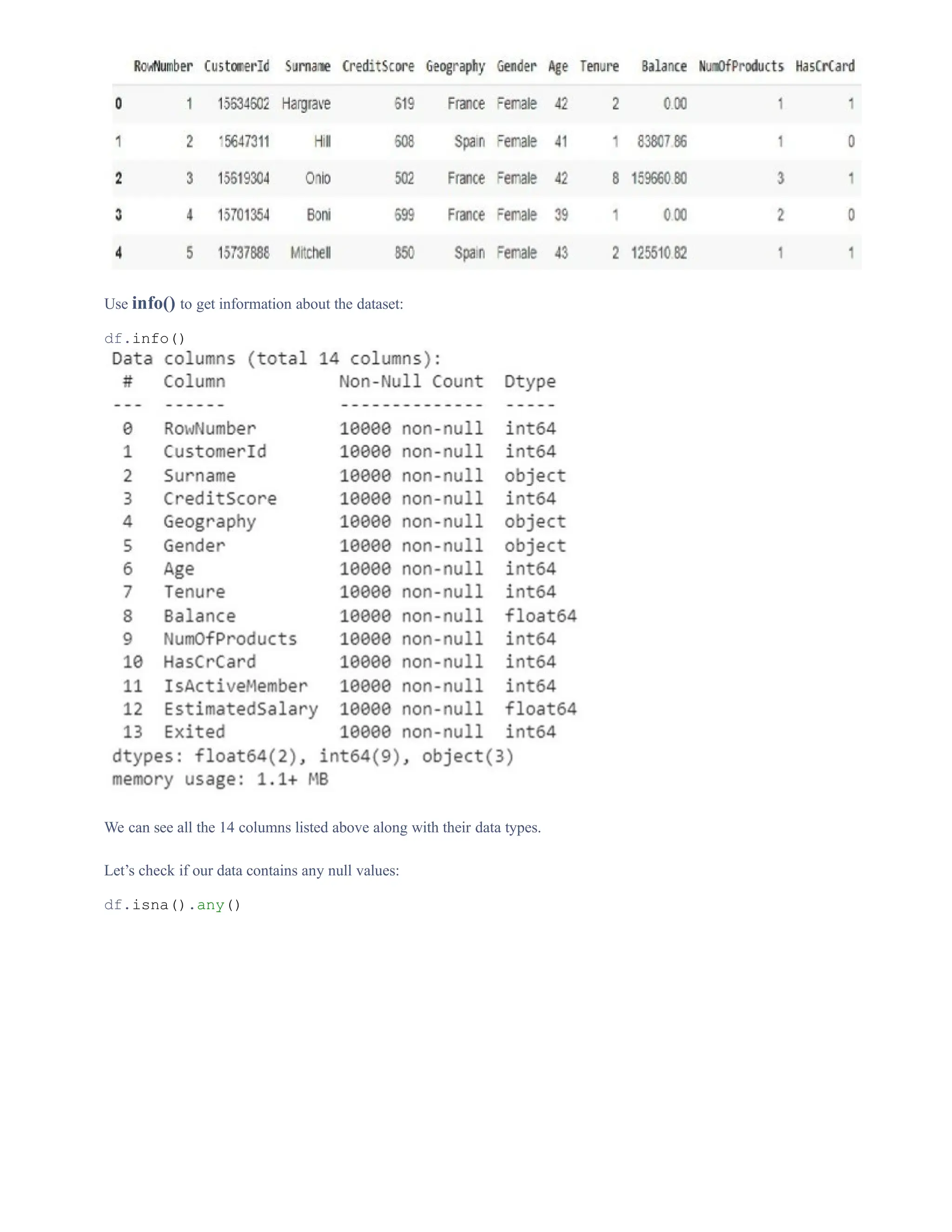
Sorting:
import pandas as pd
#Loading the dataset
df = pd.read_csv("Churn Modeling.csv")
df.head()

12. Use info() to get information about the dataset:
df.info()
We can see all the 14 columns listed above along with their data types.
Let’s check if our data contains any null values:
df.isna().any()

13. Now that it’s established that there are null values in our dataset, let’s start with understanding how sorting works in
Pandas – The pandas.sort_values() method is used to sort a DataFrame by its column or row values.
Let’s see how:
Sorting by a Column
Let’s sort our DataFrame by the ‘Balance‘ column, as shown:
balance = df.sort_values(by = 'Balance')
balance.head(10)
From what we can infer looking at the output above, is that the lowest balance is, obviously, zero.
By default, sorting always happens in ascending order, unless mentioned otherwise:
balance = df.sort_values(by = 'Balance', ascending=False)

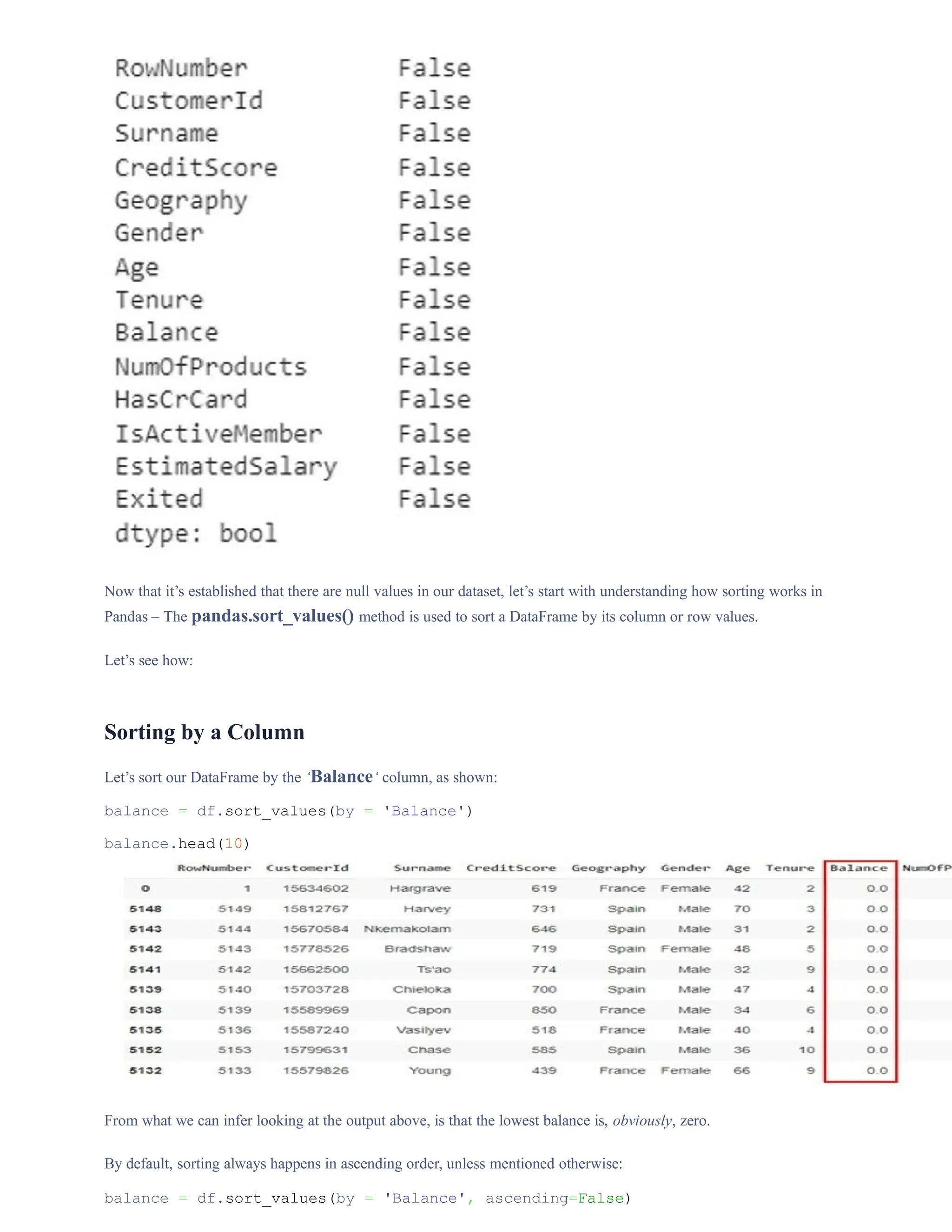
14. balance.head(10)
Sorting by Multiple Columns
We can also sort our DataFrame by more than one column at a time:
df.sort_values(by=['Geography','CreditScore']).head(10)
Sorting by multiple column with different sort orders
Sorting by Column Names
The sort_index() method can also be used to sort the DataFrame using the column names instead of rows.
For this, we need to set the axis parameter to 1:
df.sort_index(axis=1).head(10)

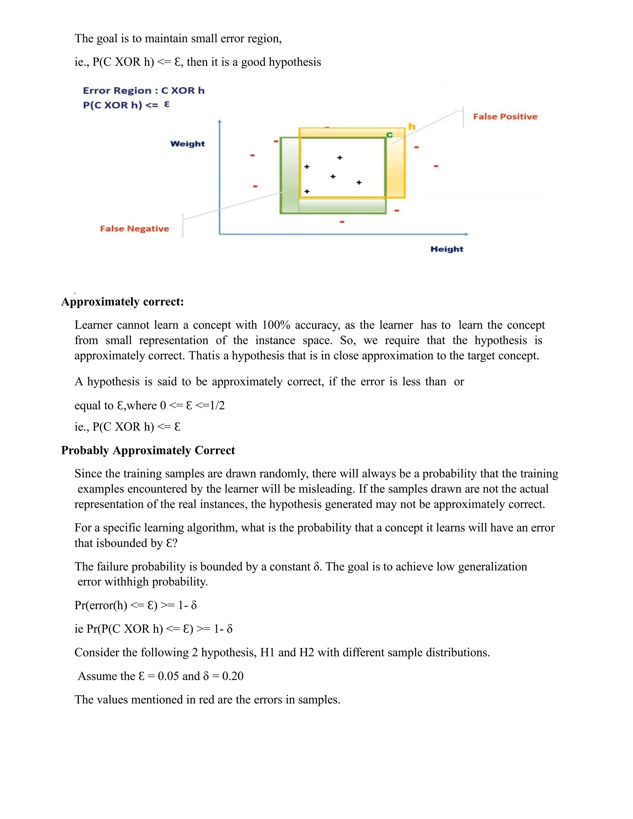
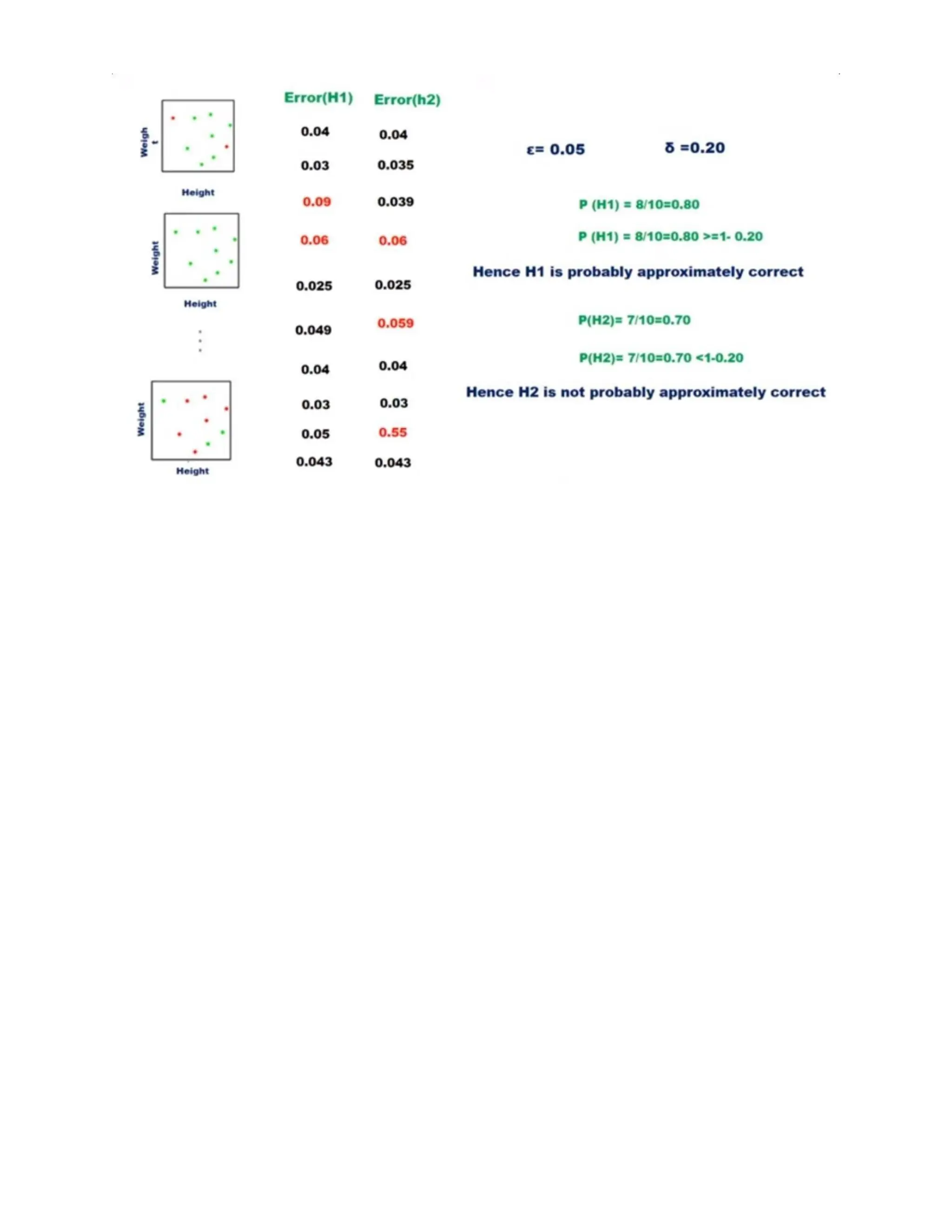
15. Probably Approximately Correct (PAC) Learning
PAC learning is a framework for the mathematical analysis of machine learning.
Goal of PAC: With high probability(“Probable”), the selected hypothesis will have lower error
(“approximately correct”)
Ɛ and δ parameters:
In the PAC model, we specify two small parameters, Ɛ and δ, and require that with probability
at least(1-δ) a system learn a concept with error at most .
Ɛ
Ɛ gives an upper bound on the error in accuracy with which h approximated (accuracy: 1- )
Ɛ
δ gives the probability of failure in achieving this accuracy (Confidence: 1-δ)
Ex: Learn the concept of “medium built person”, when given height and weight of m
individuals. Theinstance will include [height, weight] pair and the person are medium built or
not.
The following figure shows the plot of the training examples in axis aligned rectangle in 2D
plane. Theaxis aligned rectangle is the target concept.
Instances within the rectangle represents positive instances ie medium built person. Instances
outsidethe rectangle is the negative instances ie the persons are not medium built.
The learning C is unknown to the learner, so the learner generates hypothesis h that
closelyapproximates C. Since h may not be exactly same as C, results in error region.
The instances that fall within the green shaded region are all positive members according to
actual function C whereas the generated hypothesis classifies them as negative, so these
instances are calledas False Negatives.
According to C, the instances in the yellow shaded region are negative, whereas the hypothesis
classifiesthese instances as positive, so they are called as False Positives.
Error Region: C XOR h

16. The goal is to maintain small error region,
ie., P(C XOR h) <= ,
Ɛ then it is a good hypothesis
Approximately correct:
Learner cannot learn a concept with 100% accuracy, as the learner has to learn the concept
from small representation of the instance space. So, we require that the hypothesis is
approximately correct. Thatis a hypothesis that is in close approximation to the target concept.
A hypothesis is said to be approximately correct, if the error is less than or
equal to ,where
Ɛ 0 <= Ɛ <=1/2
ie., P(C XOR h) <= Ɛ
Probably Approximately Correct
Since the training samples are drawn randomly, there will always be a probability that the training
examples encountered by the learner will be misleading. If the samples drawn are not the actual
representation of the real instances, the hypothesis generated may not be approximately correct.
For a specific learning algorithm, what is the probability that a concept it learns will have an error
that isbounded by ?
Ɛ
The failure probability is bounded by a constant δ. The goal is to achieve low generalization
error withhigh probability.
Pr(error(h) <= )
Ɛ >= 1- δ
ie Pr(P(C XOR h) <= )
Ɛ >= 1- δ
Consider the following 2 hypothesis, H1 and H2 with different sample distributions.
Assume the Ɛ = 0.05 and δ = 0.20
The values mentioned in red are the errors in samples.

18. The PAC Learning Model: General Setting
Let X be the set of all possible instances over which target functions are to be defines.
C is the set of target concepts, the learner ma be asked to learn, where each c Є C, c may be
viewed as a Boolean-valued function c: X -> {0,1}
If x is a positive example c(x) = 1; if x is a negative example c(x) = 0
Examples are drawn at random from X according to a probability distribution D
A learner L considers a set of hypothesis H and, after observing some sequence of training
examples, outputs a hypothesis h Є H which is its estimate of c.
The true error of hypothesis h, w.r.t. to target concept c and distribution D is the probability that
h willmisclassify an instance drawn at random according to D
Formal Definition of PAC Learning
Consider a class C of possible target concepts defined over a set of instances X of length n, a
learner L,using hypothesis space H
C is PAC-learnable by L using H if for all c Є C, distributions D over X, Ɛ s.t., 0 < Ɛ < ½, and δ
s.t., 0 < δ <
½, learner L will output a hypothesis h Є H s.t., errorD(h) <= Ɛ with probability at least (1- δ), in
timethat is polynomial in 1/ ,
Ɛ 1/ δ, n and size(c)
Vapnik-Chervonenkis(VC) Dimension
Consider green dot as positive class and red dot as negative class. Assume we have 2 instances of
data,then these two data points can be classified into following 4 ways.

19. A line can shatter 2 points on R2
Shattering:
A set of N points is said to be shattered by a hypothesis space H, if there are hypothesis(h) in
H thatseparates positive examples from the negative examples in all of the 2N
possible ways.

20. It may not be possible to shatter every possible set of three points in 2
dimensions It is enough to find a set of three points that can be shattered.
Consider the case of 4 points, there are 16 different ways of classification. There is no single
set of 4points that can be shattered by a straight line.
Maximum number of points R2
that can be shattered by straight line is 3
So VCD(Straight line in R2
) = 3
Vapnik-Chervonenkis(VC) Dimension:
The maximum number of points that can be shattered by H is called the Vapnik-
Cherkvonenkis(VC) dimension of H. VC Dimension is one measure that characterizes the
expressive power or capacity of ahypothesis class.

21. VCD(Axis aligned rectangle):
Axis aligned rectangle cannot shatter 5 points on R2
.

22. Algorithmic steps:
Initially : G = [[?, ?, ?, ?, ?, ?], [?, ?, ?, ?, ?, ?],
[?, ?, ?, ?, ?,
?],
[?, ?, ?, ?, ?, ?], [?, ?, ?, ?, ?, ?],
[?, ?, ?, ?, ?,
?]]
S = [Null, Null, Null, Null, Null, Null]
For instance 1 : <'sunny','warm','normal','strong','warm
','same'> and positive output.
G1 = G
S1 = ['sunny','warm','normal','strong','warm
','same']
Candidate Elimination Algorithm:
The candidate elimination algorithm incrementally builds the version space given a hypothesis
space H and a set E of examples. The examples are added one by one; each example possibly
shrinks the version space by removing the hypotheses that are inconsistent with the example.
The candidate elimination algorithm does this by updating the general and specific boundary for
each new example.
 You can consider this as an extended form of the Find-S algorithm.
 Consider both positive and negative examples.
 Actually, positive examples are used here as the Find-S algorithm (Basically they are
generalizing from the specification).
 While the negative example is specified in the generalizing form.
Terms Used:
 Concept learning: Concept learning is basically the learning task of the machine (Learn by
Train data)
 General Hypothesis: Not Specifying features to learn the machine.
 G = {‘?’, ‘?’,’?’,’?’…}: Number of attributes
 Specific Hypothesis: Specifying features to learn machine (Specific feature)
 S= {‘pi’,’pi’,’pi’…}: The number of pi depends on a number of attributes.
 Version Space: It is an intermediate of general hypothesis and Specific hypothesis. It not only
just writes one hypothesis but a set of all possible hypotheses based on training data-set.
Algorithm:
Step1: Load Data set
Step2: Initialize General Hypothesis and Specific
Hypothesis.
Step3: For each training example
Step4: If example is positive example
if attribute_value == hypothesis_value:
Do
nothing
else:
replac
e
attribute
value
with '?'
(Basicall
y
generaliz
ing
it)
Step5: If example
is Negative example
Make
generalize
hypothesis
more
specific.
Example:
Consider the dataset
given below:

23. For instance 2 : <'sunny','warm','high','strong','warm
','same'> and positive output.
G2 = G
S2 = ['sunny','warm',?,'strong','warm ','same']
For instance 3 : <'rainy','cold','high','strong','warm
','change'> and negative output.
G3 = [['sunny', ?, ?, ?, ?, ?], [?,
'warm', ?, ?, ?, ?], [?,
?, ?, ?, ?, ?],
[?, ?, ?, ?, ?, ?], [?, ?, ?, ?, ?, ?],
[?, ?, ?, ?,
?, 'same']]
S3 = S2
For instance 4 :
<'sunny','warm','high','strong','cool','change'> and
positive output.
G4 = G3
S4 = ['sunny','warm',?,'strong', ?, ?]
At last, by synchronizingthe G4 and S4 algorithm produce the
output.
Output :
G = [['sunny', ?, ?, ?, ?, ?], [?, 'warm', ?, ?, ?, ?]]
S = ['sunny','warm',?,'strong', ?, ?]
The Candidate Elimination Algorithm (CEA) is an improvement over the Find-S algorithm for
classification tasks. While CEA shares some similarities with Find-S, it also has some essential
differences that offer advantages and disadvantages. Here are some advantages and
disadvantages of CEA in comparison with Find-S:
Advantages of CEA over Find-S:
1. Improved accuracy: CEA considers both positive and negative examples to generate
the hypothesis, which can result in higher accuracy when dealing with noisy or
incomplete data.
2. Flexibility: CEA can handle more complex classification tasks, such as those with multiple
classes or non-linear decision boundaries.
3. More efficient: CEA reduces the number of hypotheses by generating a set of general
hypotheses and then eliminating them one by one. This can result in faster processing and
improved efficiency.
4. Better handling of continuous attributes: CEA can handle continuous attributes by
creating boundaries for each attribute, which makes it more suitable for a wider
range of datasets.
Disadvantages of CEA in comparison with Find-S:
5. More complex: CEA is a more complex algorithm than Find-S, which may make it more
difficult for beginners or those without a strong background in machine learning to use and
understand.
6. Higher memory requirements: CEA requires more memory to store the set of hypotheses
and
boundaries, which may make it less suitable for memory-constrained environments.
3. Slower processing for large datasets: CEA may become slower for larger datasets due to
the increased number of hypotheses generated.
4. Higher potential for overfitting: The increased complexity of CEA may make it more
prone to overfitting on the training data, especially if the dataset is small or has a high
degree of noise.