Understanding Quantitative Research

1. Understanding
Quantitative
Research
Arsalan Haneef Malik

2. 2
Causation in Quantitative Research
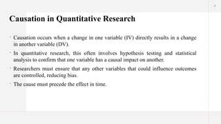
 Causation occurs when a change in one variable (IV) directly results in a change
in another variable (DV).
 In quantitative research, this often involves hypothesis testing and statistical
analysis to confirm that one variable has a causal impact on another.
 Researchers must ensure that any other variables that could influence outcomes
are controlled, reducing bias.
 The cause must precede the effect in time.

3. 3
Causation in Quantitative Research
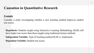
Example
Consider a study investigating whether a new teaching method improves student
test scores.
 Hypothesis: Students taught using Interactive Learning Methodology (ILM) will
have higher test scores than those taught using traditional lecture methods.
 Independent Variable: Type of teaching method (ILM vs. traditional).
 Dependent Variable: Student test scores.

4. 4
Causation in Quantitative Research
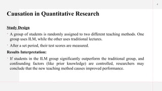
Study Design
 A group of students is randomly assigned to two different teaching methods. One
group uses ILM, while the other uses traditional lectures.
 After a set period, their test scores are measured.
Results Interpretation:
 If students in the ILM group significantly outperform the traditional group, and
confounding factors (like prior knowledge) are controlled, researchers may
conclude that the new teaching method causes improved performance.

5. 5
Description in Quantitative Research
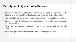
 Descriptive research emphasizes providing a detailed account of the
characteristics of a variable without inferring a cause-and-effect relationship.
 This type of research is useful for identifying patterns, trends, and demographics.
 Descriptive research often uses numerical data, surveys, or observations to outline
facts and statistics.
 There’s no experimental manipulation; researchers observe and describe what
exists.
 While findings may reveal correlations, they do not imply causation.

6. 6
Description in Quantitative Research
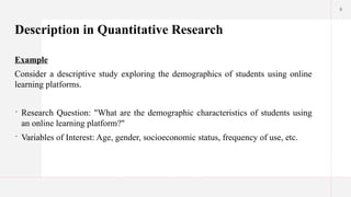
Example
Consider a descriptive study exploring the demographics of students using online
learning platforms.
 Research Question: "What are the demographic characteristics of students using
an online learning platform?"
 Variables of Interest: Age, gender, socioeconomic status, frequency of use, etc.

7. 7
Description in Quantitative Research
Study Design
 Researchers might administer a survey to collect data on students’ backgrounds and
their usage patterns of the online platform.
 The data could include categories like age ranges, gender proportions, and time
spent on the platform.
Results Interpretation:
 The results might reveal that most users are between 18-24 years old, with a
majority being female. However, while these patterns are evident, this study does
not investigate whether the demographics influence usage or outcomes. It merely
describes who is using the platform.

8. 8
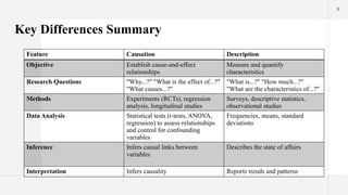
Key Differences Summary
Feature Causation Description
Objective Establish cause-and-effect
relationships
Measure and quantify
characteristics
Research Questions "Why...?" "What is the effect of...?"
"What causes...?"
"What is...?" "How much...?"
"What are the characteristics of...?"
Methods Experiments (RCTs), regression
analysis, longitudinal studies
Surveys, descriptive statistics,
observational studies
Data Analysis Statistical tests (t-tests, ANOVA,
regression) to assess relationships
and control for confounding
variables
Frequencies, means, standard
deviations
Inference Infers causal links between
variables
Describes the state of affairs
Interpretation Infers causality Reports trends and patterns

9. 9
Important Considerations
 Correlation does not equal causation: Just because two variables are correlated
doesn't mean one causes the other. There might be a third, unmeasured variable
influencing both.
 Establishing causality is challenging: It requires careful experimental design and
strong evidence to rule out alternative explanations.
 Quantitative methods are suited for both: While certain designs are better
suited to causal inferences, both descriptive and causal questions can be addressed
using quantitative methods.

10. 10
Measurement
 Measurement is the process of assigning numbers or labels to observations
according to a set of rules.
 These rules define how the characteristic being measured (the variable) is
quantified.
 The quality of your measurement directly impacts the validity and reliability of
your findings.

11. 11
Measurement (Types)
 Nominal: Data is categorized without a specific order (e.g., gender, race).
 Ordinal: Data is categorized in a specific order but does not have a consistent
difference between categories (e.g., rankings in a competition).
 Interval: Data has meaningful differences between values but no true zero point
(e.g., temperature in Celsius).
 Ratio: Data has a true zero point, allowing for meaningful comparisons (e.g.,
height, weight, age).

12. 12
Measurement (Examples)
If a researcher wants to measure academic performance:
 The researcher could assign grades (A, B, C) – nominal measurement.
 Alternatively, they could use test scores (0-100) – ratio measurement.
 Measuring height with a ruler (a straightforward, well-defined measurement).
 Measuring intelligence with an IQ test (a more complex measurement, subject to
interpretation).
 Measuring customer satisfaction with a survey (measurement involves assigning
numerical scores to responses, potentially using Likert scales).
 Measuring blood pressure with a sphygmomanometer (a precise instrument providing
quantitative data).

13. 13
Validity
Validity refers to the extent to which a measurement accurately represents the
concept it intends to measure. It assesses whether the research instrument (like a
survey or test) truly measures what it claims to measure.

14. 14
Validity (Types)
Content Validity:
 Does the measurement instrument cover all the relevant aspects of the construct
being measured?
 Ensures that the measurement covers the entire domain of the concept
Criterion Validity:
 Does the measurement correlate with an established criterion or gold standard?
 For instance, a new blood pressure measurement device's readings should
correlate highly with readings from a well-established device.

15. 15
Validity (Types)
Criterion Validity
There are two main types of criterion validity
Concurrent Validity: This is like comparing your new thermometer to a trusted
one at the same time. We measure both the new test and the gold standard at the
same point, and see if they correlate.
Predictive Validity: This is like using your new thermometer to predict future
weather patterns. We use the new test to predict a future outcome, and then compare
that prediction to what actually happens.
In short, criterion validity ensures that our tests and measurements are accurate
and meaningful. It helps us make sure that we're measuring what we think we're
measuring.

16. 16
Validity (Types)
Construct Validity:
 Does the measurement instrument accurately reflect the underlying theoretical
construct?
 This is often assessed through convergent validity (correlation with similar
measures) and discriminant validity (lack of correlation with dissimilar measures).
 For example, a test measuring "extraversion" should correlate with other measures
of extraversion but not with measures of introversion.
In short, construct validity ensures that your measurement tool accurately captures
the abstract concept you're interested in. It's about making sure you're measuring the
right thing in the right way.

17. 17
Reliability
Reliability refers to the consistency and stability of a measurement over time. A
reliable instrument yields the same results under consistent conditions. It is crucial for
ensuring that the measurement does not fluctuate due to random error.
 Test-retest reliability: Consistency of scores over time. If you administer the same
test to the same individuals at two different times, the scores should be similar.
 Inter-rater reliability: Consistency of scores across different raters or observers. If
multiple people rate the same observation, their ratings should be similar.
 Internal consistency reliability: Consistency of scores within a single test or
instrument. This is often assessed using Cronbach's alpha for questionnaires,
indicating the extent to which items within the scale measure the same construct.

18. 18
Constructs Operationalization
 Construct operationalization is the process of defining a theoretical construct (an
abstract concept) in concrete, measurable terms.
 In simpler words, it's bridging the gap between an abstract idea and its empirical
representation.
 This is crucial because you can't directly measure abstract concepts like
"intelligence," "happiness," or "customer satisfaction."
 A researcher need to define them in ways that allow for observation and
quantification.

19. 19
Constructs
Constructs are abstract concepts or variables that researchers want to study but
cannot directly measure.
 Intelligence: Not directly observable, but inferred from performance on cognitive
tasks.
 Motivation: Inferred from behaviours like effort, persistence, and goal-directed
actions.
 Stress: Inferred from physiological measures (heart rate, cortisol levels), self-
reported feelings, and behavioural changes.
 Brand loyalty: Inferred from repeated purchasing behaviour, positive word-of-
mouth, and emotional attachment to a brand.

20. 20
Operationalization: Turning Constructs into
Measurable Variables
Operationalization involves specifying the observable indicators or behaviours that
will be used to represent the construct. This involves defining how the construct will
be measured.
The process typically involves several steps:
 Conceptual Definition: Start with a clear, concise definition of the construct
based on existing literature and theory. This establishes the theoretical meaning of
the construct.
 Selection of Indicators: Identify specific, observable behaviours, responses, or
measures that reflect the construct. The choice of indicators depends on the
research question and the nature of the construct.

21. 21
Operationalization
 Development of Measurement Instruments: Develop or select a tool
(questionnaire, scale, experiment, observation checklist, etc.) to collect data on the
chosen indicators. This might involve creating questions, selecting existing scales,
or designing an experiment to elicit relevant behaviours.
 Data Collection: Use the chosen instrument to collect data from participants or
subjects.

22. 22
Operationalization
 Pilot Testing: Conduct a pilot test of the measurement instruments to identify any
potential issues with the questions, clarity, and understanding from participants.
Make necessary revisions based on feedback.
 Example: Before the main study, a smaller group could complete the anxiety
questionnaire, and researchers could adjust ambiguous wording based on
participants' feedback.
 Data Analysis: Analyse the collected data using appropriate statistical techniques
to quantify the construct and test hypotheses.

23. 23
Operationalization
 For the process, refer to the handout.

24. 24
Descriptive Stats

25. 25
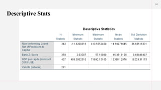
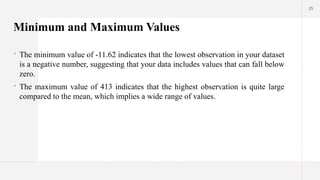
Minimum and Maximum Values
 The minimum value of -11.62 indicates that the lowest observation in your dataset
is a negative number, suggesting that your data includes values that can fall below
zero.
 The maximum value of 413 indicates that the highest observation is quite large
compared to the mean, which implies a wide range of values.

26. 26
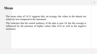
Mean
 The mean value of 14.11 suggests that, on average, the values in the dataset are
relatively low compared to the maximum.
 This indicates that the central tendency of the data is near 14, but this average is
influenced by the presence of higher values (like 413) as well as the negative
minimum.

27. 27
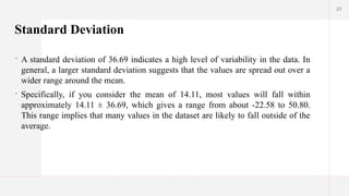
Standard Deviation
 A standard deviation of 36.69 indicates a high level of variability in the data. In
general, a larger standard deviation suggests that the values are spread out over a
wider range around the mean.
 Specifically, if you consider the mean of 14.11, most values will fall within
approximately 14.11 ± 36.69, which gives a range from about -22.58 to 50.80.
This range implies that many values in the dataset are likely to fall outside of the
average.

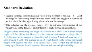
28. Standard Deviation
 Because the range includes negative values while the mean is positive (14.11), and
the range is substantially larger than the mean itself, this suggests a substantial
portion of the data lies significantly above or below the average.
 This indicates that the average value (14.11) is not very representative of the
typical value in the dataset. The distribution is likely skewed or has outliers.
Imagine you're measuring the height of students in a class. The average height
might be 5 feet (the mean). However, if the standard deviation is very large (like 2
feet), it means some students are incredibly tall (perhaps 7 feet) and some are very
short (maybe 3 feet). The average height of 5 feet doesn't really capture the typical
height well because the data is so spread out. This is what the statement is
conveying – the mean doesn't represent the data well due to high variability.

29. 29
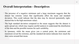
Overall Interpretation - Descriptives
 The presence of a negative minimum and a large maximum suggests that the
dataset has extreme values that significantly affect the mean and standard
deviation. This could indicate that the data may be skewed (potentially right-
skewed due to the high maximum value).
 The high standard deviation compared to the mean suggests that the dataset is
quite spread out, which may require careful analysis to understand the distribution
of the data and the possible reasons for such variability.
 In summary, while the mean gives you a central point, the minimum and
maximum reveal the extremes, and the standard deviation indicates how much the
data varies around that mean.

30. Correlation Analysis

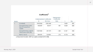
31. 31
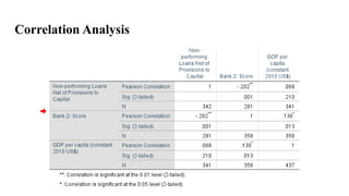
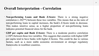
Overall Interpretation - Correlation
 Non-performing Loans and Bank Z-Score: There is a strong negative
correlation (-.202**) between these two variables. This means that as the ratio of
non-performing loans to capital increases, the bank's Z-Score tends to decrease.
This makes intuitive sense, as a higher proportion of non-performing loans
indicates potential financial stress for the bank.
 GDP per capita and Bank Z-Score: There is a moderate positive correlation
(.130*) between these two variables. This suggests that countries with higher GDP
per capita tend to have banks with higher Z-Scores. This could be due to various
factors, such as a more stable economic environment or stronger regulatory
frameworks in wealthier countries.

32. 32
Regression Analysis (Simple)

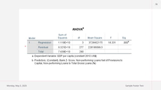
33. 33
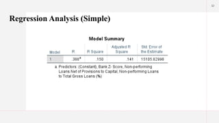
Model Fitness
 R-squared measures the proportion of the variance in the dependent variable that
can be explained by the independent variables in the model.
 Range: R-squared values range from 0 to 1. A value of 0 means that none of the
variance is explained by the model, while a value of 1 means that all the variance
is explained perfectly.

34. 34
Model Fitness
 Adjusted R-squared modifies R-squared to account for the number of predictors in
the model. It adjusts the R-squared value based on how many independent variables
are included in the model and the sample size.
 Range: Adjusted R-squared can be less than 0 or greater than R-squared, and it can
decrease if unnecessary predictors are added. This makes it a more reliable measure
when comparing models with different numbers of independent variables.
 Usefulness: Adjusted R-squared is especially useful when you want to determine
whether adding additional variables improves the model significantly. If adjusted R-
squared increases, it indicates that the new variable contributes to explaining the
response variable. If it decreases, it suggests that the new variable does not improve
the model.

35. 35
Model Fitness
 Adjusted R-squared modifies R-squared to account for the number of predictors in
the model. It adjusts the R-squared value based on how many independent variables
are included in the model and the sample size.
 Range: Adjusted R-squared can be less than 0 or greater than R-squared, and it can
decrease if unnecessary predictors are added. This makes it a more reliable measure
when comparing models with different numbers of independent variables.
 Usefulness: Adjusted R-squared is especially useful when you want to determine
whether adding additional variables improves the model significantly. If adjusted R-
squared increases, it indicates that the new variable contributes to explaining the
response variable. If it decreases, it suggests that the new variable does not improve
the model.

36. Monday, May 5, 2025 Sample Footer Text
36

37. Monday, May 5, 2025 Sample Footer Text
37