Joris Van Den Bossche (Ghent University): “Introduction to Pandas” Abstract: Pandas is becoming the fundamental library for manipulating and analyzing structured data, providing high-performance, easy-to-use data structures and data analysis tools. This talk will give a basic introduction to pandas, explaining the key concepts and defining features. Bio: I am a PhD student at Ghent University (Department of Mathematical Modelling, Statistics and Bio-informatics) working on mobile air quality monitoring in collaboration with VITO (Flemish Institute for Technological Research). I am also a contributor to pandas, and since a year a member of the core development team.

1. Introduction to Pandas
April 3rd, 2015
Joris Van den Bossche
Source: https://github.com/jorisvandenbossche/2015-PyDataParis

2. About me: Joris Van den Bossche
PhD student at Ghent University and VITO, Belgium
bio-science engineer, air quality research
pandas core dev
->
Licensed under
https://github.com/jorisvandenbossche (https://github.com/jorisvandenbossche)
@jorisvdbossche (https://twitter.com/jorisvdbossche)
CC BY 4.0 Creative Commons (http://creativecommons.org/licenses/by/4.0/)

3. Content of this talk
Why do you need pandas?
Basic introduction to the data structures
Guided tour through some of the pandas features with a case study
If you want to follow along, this is a notebook that you can view or run yourself:
All materials (notebook, data, link to nbviewer):
You need p
a
n
d
a
s
> 0.15 (easy solution is using Anaconda)
https://github.com/jorisvandenbossche/2015-PyDataParis
(https://github.com/jorisvandenbossche/2015-PyDataParis)

4. Some imports:
I
n
[
1
]
: %
m
a
t
p
l
o
t
l
i
b i
n
l
i
n
e
i
m
p
o
r
t p
a
n
d
a
s a
s p
d
i
m
p
o
r
t n
u
m
p
y a
s n
p
i
m
p
o
r
t m
a
t
p
l
o
t
l
i
b
.
p
y
p
l
o
t a
s p
l
t
i
m
p
o
r
t s
e
a
b
o
r
n
p
d
.
o
p
t
i
o
n
s
.
d
i
s
p
l
a
y
.
m
a
x
_
r
o
w
s = 8

5. Let's start with a showcase

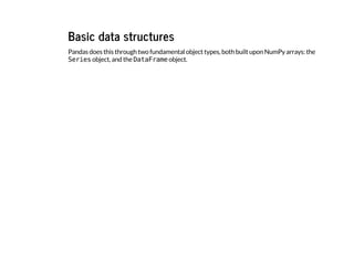
6. Case study: air quality in Europe
AirBase (The European Air quality dataBase): hourly measurements of all air quality
monitoring stations from Europe
Starting from these hourly data for different stations:
I
n
[
3
]
: d
a
t
a
O
u
t
[
3
]
: BETR801 BETN029 FR04037 FR04012
1990-01-01 00:00:00 NaN 16.0 NaN NaN
1990-01-01 01:00:00 NaN 18.0 NaN NaN
1990-01-01 02:00:00 NaN 21.0 NaN NaN
1990-01-01 03:00:00 NaN 26.0 NaN NaN
... ... ... ... ...
2012-12-31 20:00:00 16.5 2.0 16 47
2012-12-31 21:00:00 14.5 2.5 13 43
2012-12-31 22:00:00 16.5 3.5 14 42
2012-12-31 23:00:00 15.0 3.0 13 49
198895 rows × 4 columns

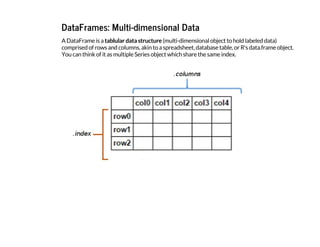
7. to answering questions about this data in a few lines of code:
Does the air pollution show a decreasing trend over the years?
I
n
[
4
]
: d
a
t
a
[
'
1
9
9
9
'
:
]
.
r
e
s
a
m
p
l
e
(
'
A
'
)
.
p
l
o
t
(
y
l
i
m
=
[
0
,
1
0
0
]
)
O
u
t
[
4
]
: <
m
a
t
p
l
o
t
l
i
b
.
a
x
e
s
.
_
s
u
b
p
l
o
t
s
.
A
x
e
s
S
u
b
p
l
o
t a
t 0
x
a
a
c
4
6
9
e
c
>

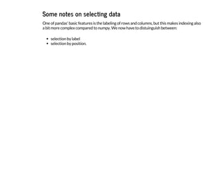
8. How many exceedances of the limit values?
I
n
[
5
]
: e
x
c
e
e
d
a
n
c
e
s = d
a
t
a > 2
0
0
e
x
c
e
e
d
a
n
c
e
s = e
x
c
e
e
d
a
n
c
e
s
.
g
r
o
u
p
b
y
(
e
x
c
e
e
d
a
n
c
e
s
.
i
n
d
e
x
.
y
e
a
r
)
.
s
u
m
(
)
a
x = e
x
c
e
e
d
a
n
c
e
s
.
l
o
c
[
2
0
0
5
:
]
.
p
l
o
t
(
k
i
n
d
=
'
b
a
r
'
)
a
x
.
a
x
h
l
i
n
e
(
1
8
, c
o
l
o
r
=
'
k
'
, l
i
n
e
s
t
y
l
e
=
'
-
-
'
)
O
u
t
[
5
]
: <
m
a
t
p
l
o
t
l
i
b
.
l
i
n
e
s
.
L
i
n
e
2
D a
t 0
x
a
a
c
4
6
3
6
c
>

9. What is the difference in diurnal profile between weekdays and weekend?
I
n
[
6
]
: d
a
t
a
[
'
w
e
e
k
d
a
y
'
] = d
a
t
a
.
i
n
d
e
x
.
w
e
e
k
d
a
y
d
a
t
a
[
'
w
e
e
k
e
n
d
'
] = d
a
t
a
[
'
w
e
e
k
d
a
y
'
]
.
i
s
i
n
(
[
5
, 6
]
)
d
a
t
a
_
w
e
e
k
e
n
d = d
a
t
a
.
g
r
o
u
p
b
y
(
[
'
w
e
e
k
e
n
d
'
, d
a
t
a
.
i
n
d
e
x
.
h
o
u
r
]
)
[
'
F
R
0
4
0
1
2
'
]
.
m
e
a
n
(
)
.
u
n
s
t
a
c
k
(
l
e
v
e
l
=
0
)
d
a
t
a
_
w
e
e
k
e
n
d
.
p
l
o
t
(
)
O
u
t
[
6
]
: <
m
a
t
p
l
o
t
l
i
b
.
a
x
e
s
.
_
s
u
b
p
l
o
t
s
.
A
x
e
s
S
u
b
p
l
o
t a
t 0
x
a
b
3
7
3
6
2
c
>
We will come back to these example, and build them up step by step.

10. Why do you need pandas?

11. Why do you need pandas?
When working with tabular or structured data (like R dataframe, SQL table, Excel spreadsheet,
...):
Import data
Clean up messy data
Explore data, gain insight into data
Process and prepare your data for analysis
Analyse your data (together with scikit-learn, statsmodels, ...)

12. Pandas: data analysis in python
For data-intensive work in Python the library has become
essential.
What is p
a
n
d
a
s
?
Pandas can be thought of as NumPy arrays with labels for rows and columns, and
better support for heterogeneous data types, but it's also much, much more than
that.
Pandas can also be thought of as R
's d
a
t
a
.
f
r
a
m
e
in Python.
Powerful for working with missing data, working with time series data, for reading
and writing your data, for reshaping, grouping, merging your data, ...
It's documentation:
Pandas (http://pandas.pydata.org)
http://pandas.pydata.org/pandas-docs/stable/
(http://pandas.pydata.org/pandas-docs/stable/)

13. Key features
Fast, easy and flexible input/output for a lot of different data formats
Working with missing data (.
d
r
o
p
n
a
(
)
, p
d
.
i
s
n
u
l
l
(
)
)
Merging and joining (c
o
n
c
a
t
, j
o
i
n
)
Grouping: g
r
o
u
p
b
y
functionality
Reshaping (s
t
a
c
k
, p
i
v
o
t
)
Powerful time series manipulation (resampling, timezones, ..)
Easy plotting

14. Basic data structures
Pandas does this through two fundamental object types, both built upon NumPy arrays: the
S
e
r
i
e
s
object, and the D
a
t
a
F
r
a
m
e
object.

15. Series
A Series is a basic holder for one-dimensional labeled data. It can be created much as a NumPy
array is created:
I
n
[
7
]
: s = p
d
.
S
e
r
i
e
s
(
[
0
.
1
, 0
.
2
, 0
.
3
, 0
.
4
]
)
s
O
u
t
[
7
]
: 0 0
.
1
1 0
.
2
2 0
.
3
3 0
.
4
d
t
y
p
e
: f
l
o
a
t
6
4

16. Attributes of a Series: i
n
d
e
xand v
a
l
u
e
s
The series has a built-in concept of an index, which by default is the numbers 0 through N - 1
I
n
[
8
]
: s
.
i
n
d
e
x
O
u
t
[
8
]
: I
n
t
6
4
I
n
d
e
x
(
[
0
, 1
, 2
, 3
]
, d
t
y
p
e
=
'
i
n
t
6
4
'
)
You can access the underlying numpy array representation with the .
v
a
l
u
e
s
attribute:
I
n
[
9
]
: s
.
v
a
l
u
e
s
O
u
t
[
9
]
: a
r
r
a
y
(
[ 0
.
1
, 0
.
2
, 0
.
3
, 0
.
4
]
)

17. We can access series values via the index, just like for NumPy arrays:
I
n
[
1
0
]
: s
[
0
]
O
u
t
[
1
0
]
: 0
.
1
0
0
0
0
0
0
0
0
0
0
0
0
0
0
0
1

18. Unlike the NumPy array, though, this index can be something other than integers:
I
n
[
1
1
]
: s
2 = p
d
.
S
e
r
i
e
s
(
n
p
.
a
r
a
n
g
e
(
4
)
, i
n
d
e
x
=
[
'
a
'
, '
b
'
, '
c
'
, '
d
'
]
)
s
2
O
u
t
[
1
1
]
: a 0
b 1
c 2
d 3
d
t
y
p
e
: i
n
t
3
2
I
n
[
1
2
]
: s
2
[
'
c
'
]
O
u
t
[
1
2
]
: 2

19. In this way, a S
e
r
i
e
s
object can be thought of as similar to an ordered dictionary mapping one
typed value to another typed value:
I
n
[
1
3
]
: p
o
p
u
l
a
t
i
o
n = p
d
.
S
e
r
i
e
s
(
{
'
G
e
r
m
a
n
y
'
: 8
1
.
3
, '
B
e
l
g
i
u
m
'
: 1
1
.
3
, '
F
r
a
n
c
e
'
: 6
4
.
3
, '
U
n
i
t
e
d K
i
n
g
d
o
m
'
: 6
4
.
9
, '
N
e
t
h
e
r
l
a
n
d
s
'
: 1
6
.
9
}
)
p
o
p
u
l
a
t
i
o
n
O
u
t
[
1
3
]
: B
e
l
g
i
u
m 1
1
.
3
F
r
a
n
c
e 6
4
.
3
G
e
r
m
a
n
y 8
1
.
3
N
e
t
h
e
r
l
a
n
d
s 1
6
.
9
U
n
i
t
e
d K
i
n
g
d
o
m 6
4
.
9
d
t
y
p
e
: f
l
o
a
t
6
4
I
n
[
1
4
]
: p
o
p
u
l
a
t
i
o
n
[
'
F
r
a
n
c
e
'
]
O
u
t
[
1
4
]
: 6
4
.
2
9
9
9
9
9
9
9
9
9
9
9
9
9
7
but with the power of numpy arrays:
I
n
[
1
5
]
: p
o
p
u
l
a
t
i
o
n * 1
0
0
0
O
u
t
[
1
5
]
: B
e
l
g
i
u
m 1
1
3
0
0
F
r
a
n
c
e 6
4
3
0
0
G
e
r
m
a
n
y 8
1
3
0
0
N
e
t
h
e
r
l
a
n
d
s 1
6
9
0
0
U
n
i
t
e
d K
i
n
g
d
o
m 6
4
9
0
0
d
t
y
p
e
: f
l
o
a
t
6
4

20. We can index or slice the populations as expected:
I
n
[
1
6
]
: p
o
p
u
l
a
t
i
o
n
[
'
B
e
l
g
i
u
m
'
]
O
u
t
[
1
6
]
: 1
1
.
3
0
0
0
0
0
0
0
0
0
0
0
0
0
1
I
n
[
1
7
]
: p
o
p
u
l
a
t
i
o
n
[
'
B
e
l
g
i
u
m
'
:
'
G
e
r
m
a
n
y
'
]
O
u
t
[
1
7
]
: B
e
l
g
i
u
m 1
1
.
3
F
r
a
n
c
e 6
4
.
3
G
e
r
m
a
n
y 8
1
.
3
d
t
y
p
e
: f
l
o
a
t
6
4

21. Many things you can do with numpy arrays, can also be applied on objects.
Fancy indexing, like indexing with a list or boolean indexing:
I
n
[
1
8
]
: p
o
p
u
l
a
t
i
o
n
[
[
'
F
r
a
n
c
e
'
, '
N
e
t
h
e
r
l
a
n
d
s
'
]
]
O
u
t
[
1
8
]
: F
r
a
n
c
e 6
4
.
3
N
e
t
h
e
r
l
a
n
d
s 1
6
.
9
d
t
y
p
e
: f
l
o
a
t
6
4
I
n
[
1
9
]
: p
o
p
u
l
a
t
i
o
n
[
p
o
p
u
l
a
t
i
o
n > 2
0
]
O
u
t
[
1
9
]
: F
r
a
n
c
e 6
4
.
3
G
e
r
m
a
n
y 8
1
.
3
U
n
i
t
e
d K
i
n
g
d
o
m 6
4
.
9
d
t
y
p
e
: f
l
o
a
t
6
4

22. Element-wise operations:
I
n
[
2
0
]
: p
o
p
u
l
a
t
i
o
n / 1
0
0
O
u
t
[
2
0
]
: B
e
l
g
i
u
m 0
.
1
1
3
F
r
a
n
c
e 0
.
6
4
3
G
e
r
m
a
n
y 0
.
8
1
3
N
e
t
h
e
r
l
a
n
d
s 0
.
1
6
9
U
n
i
t
e
d K
i
n
g
d
o
m 0
.
6
4
9
d
t
y
p
e
: f
l
o
a
t
6
4
A range of methods:
I
n
[
2
1
]
: p
o
p
u
l
a
t
i
o
n
.
m
e
a
n
(
)
O
u
t
[
2
1
]
: 4
7
.
7
3
9
9
9
9
9
9
9
9
9
9
9
9
5

23. Alignment!
Only, pay attention to alignment: operations between series will align on the index:
I
n
[
2
2
]
: s
1 = p
o
p
u
l
a
t
i
o
n
[
[
'
B
e
l
g
i
u
m
'
, '
F
r
a
n
c
e
'
]
]
s
2 = p
o
p
u
l
a
t
i
o
n
[
[
'
F
r
a
n
c
e
'
, '
G
e
r
m
a
n
y
'
]
]
I
n
[
2
3
]
: s
1
O
u
t
[
2
3
]
: B
e
l
g
i
u
m 1
1
.
3
F
r
a
n
c
e 6
4
.
3
d
t
y
p
e
: f
l
o
a
t
6
4
I
n
[
2
4
]
: s
2
O
u
t
[
2
4
]
: F
r
a
n
c
e 6
4
.
3
G
e
r
m
a
n
y 8
1
.
3
d
t
y
p
e
: f
l
o
a
t
6
4
I
n
[
2
5
]
: s
1 + s
2
O
u
t
[
2
5
]
: B
e
l
g
i
u
m N
a
N
F
r
a
n
c
e 1
2
8
.
6
G
e
r
m
a
n
y N
a
N
d
t
y
p
e
: f
l
o
a
t
6
4

24. DataFrames: Multi-dimensional Data
A DataFrame is a tablular data structure (multi-dimensional object to hold labeled data)
comprised of rows and columns, akin to a spreadsheet, database table, or R's data.frame object.
You can think of it as multiple Series object which share the same index.

25. One of the most common ways of creating a dataframe is from a dictionary of arrays or lists.
Note that in the IPython notebook, the dataframe will display in a rich HTML view:
I
n
[
2
6
]
: d
a
t
a = {
'
c
o
u
n
t
r
y
'
: [
'
B
e
l
g
i
u
m
'
, '
F
r
a
n
c
e
'
, '
G
e
r
m
a
n
y
'
, '
N
e
t
h
e
r
l
a
n
d
s
'
, '
U
n
i
t
e
d K
i
n
g
d
o
m
'
]
,
'
p
o
p
u
l
a
t
i
o
n
'
: [
1
1
.
3
, 6
4
.
3
, 8
1
.
3
, 1
6
.
9
, 6
4
.
9
]
,
'
a
r
e
a
'
: [
3
0
5
1
0
, 6
7
1
3
0
8
, 3
5
7
0
5
0
, 4
1
5
2
6
, 2
4
4
8
2
0
]
,
'
c
a
p
i
t
a
l
'
: [
'
B
r
u
s
s
e
l
s
'
, '
P
a
r
i
s
'
, '
B
e
r
l
i
n
'
, '
A
m
s
t
e
r
d
a
m
'
, '
L
o
n
d
o
n
'
]
}
c
o
u
n
t
r
i
e
s = p
d
.
D
a
t
a
F
r
a
m
e
(
d
a
t
a
)
c
o
u
n
t
r
i
e
s
O
u
t
[
2
6
]
: area capital country population
0 30510 Brussels Belgium 11.3
1 671308 Paris France 64.3
2 357050 Berlin Germany 81.3
3 41526 Amsterdam Netherlands 16.9
4 244820 London United Kingdom 64.9

26. Attributes of the DataFrame
A DataFrame has besides a i
n
d
e
x
attribute, also a c
o
l
u
m
n
s
attribute:
I
n
[
2
7
]
: c
o
u
n
t
r
i
e
s
.
i
n
d
e
x
O
u
t
[
2
7
]
: I
n
t
6
4
I
n
d
e
x
(
[
0
, 1
, 2
, 3
, 4
]
, d
t
y
p
e
=
'
i
n
t
6
4
'
)
I
n
[
2
8
]
: c
o
u
n
t
r
i
e
s
.
c
o
l
u
m
n
s
O
u
t
[
2
8
]
: I
n
d
e
x
(
[
u
'
a
r
e
a
'
, u
'
c
a
p
i
t
a
l
'
, u
'
c
o
u
n
t
r
y
'
, u
'
p
o
p
u
l
a
t
i
o
n
'
]
, d
t
y
p
e
=
'
o
b
j
e
c
t
'
)

27. To check the data types of the different columns:
I
n
[
2
9
]
: c
o
u
n
t
r
i
e
s
.
d
t
y
p
e
s
O
u
t
[
2
9
]
: a
r
e
a i
n
t
6
4
c
a
p
i
t
a
l o
b
j
e
c
t
c
o
u
n
t
r
y o
b
j
e
c
t
p
o
p
u
l
a
t
i
o
n f
l
o
a
t
6
4
d
t
y
p
e
: o
b
j
e
c
t

28. An overview of that information can be given with the i
n
f
o
(
)
method:
I
n
[
3
0
]
: c
o
u
n
t
r
i
e
s
.
i
n
f
o
(
)
<
c
l
a
s
s '
p
a
n
d
a
s
.
c
o
r
e
.
f
r
a
m
e
.
D
a
t
a
F
r
a
m
e
'
>
I
n
t
6
4
I
n
d
e
x
: 5 e
n
t
r
i
e
s
, 0 t
o 4
D
a
t
a c
o
l
u
m
n
s (
t
o
t
a
l 4 c
o
l
u
m
n
s
)
:
a
r
e
a 5 n
o
n
-
n
u
l
l i
n
t
6
4
c
a
p
i
t
a
l 5 n
o
n
-
n
u
l
l o
b
j
e
c
t
c
o
u
n
t
r
y 5 n
o
n
-
n
u
l
l o
b
j
e
c
t
p
o
p
u
l
a
t
i
o
n 5 n
o
n
-
n
u
l
l f
l
o
a
t
6
4
d
t
y
p
e
s
: f
l
o
a
t
6
4
(
1
)
, i
n
t
6
4
(
1
)
, o
b
j
e
c
t
(
2
)
m
e
m
o
r
y u
s
a
g
e
: 1
6
0
.
0
+ b
y
t
e
s

29. Also a DataFrame has a v
a
l
u
e
s
attribute, but attention: when you have heterogeneous data,
all values will be upcasted:
I
n
[
3
1
]
: c
o
u
n
t
r
i
e
s
.
v
a
l
u
e
s
O
u
t
[
3
1
]
: a
r
r
a
y
(
[
[
3
0
5
1
0
L
, '
B
r
u
s
s
e
l
s
'
, '
B
e
l
g
i
u
m
'
, 1
1
.
3
]
,
[
6
7
1
3
0
8
L
, '
P
a
r
i
s
'
, '
F
r
a
n
c
e
'
, 6
4
.
3
]
,
[
3
5
7
0
5
0
L
, '
B
e
r
l
i
n
'
, '
G
e
r
m
a
n
y
'
, 8
1
.
3
]
,
[
4
1
5
2
6
L
, '
A
m
s
t
e
r
d
a
m
'
, '
N
e
t
h
e
r
l
a
n
d
s
'
, 1
6
.
9
]
,
[
2
4
4
8
2
0
L
, '
L
o
n
d
o
n
'
, '
U
n
i
t
e
d K
i
n
g
d
o
m
'
, 6
4
.
9
]
]
, d
t
y
p
e
=
o
b
j
e
c
t
)

30. If we don't like what the index looks like, we can reset it and set one of our columns:
I
n
[
3
2
]
: c
o
u
n
t
r
i
e
s = c
o
u
n
t
r
i
e
s
.
s
e
t
_
i
n
d
e
x
(
'
c
o
u
n
t
r
y
'
)
c
o
u
n
t
r
i
e
s
O
u
t
[
3
2
]
: area capital population
country
Belgium 30510 Brussels 11.3
France 671308 Paris 64.3
Germany 357050 Berlin 81.3
Netherlands 41526 Amsterdam 16.9
United Kingdom 244820 London 64.9

31. To access a Series representing a column in the data, use typical indexing syntax:
I
n
[
3
3
]
: c
o
u
n
t
r
i
e
s
[
'
a
r
e
a
'
]
O
u
t
[
3
3
]
: c
o
u
n
t
r
y
B
e
l
g
i
u
m 3
0
5
1
0
F
r
a
n
c
e 6
7
1
3
0
8
G
e
r
m
a
n
y 3
5
7
0
5
0
N
e
t
h
e
r
l
a
n
d
s 4
1
5
2
6
U
n
i
t
e
d K
i
n
g
d
o
m 2
4
4
8
2
0
N
a
m
e
: a
r
e
a
, d
t
y
p
e
: i
n
t
6
4

32. As you play around with DataFrames, you'll notice that many operations which work on
NumPy arrays will also work on dataframes.
Let's compute density of each country:
I
n
[
3
4
]
: c
o
u
n
t
r
i
e
s
[
'
p
o
p
u
l
a
t
i
o
n
'
]
*
1
0
0
0
0
0
0 / c
o
u
n
t
r
i
e
s
[
'
a
r
e
a
'
]
O
u
t
[
3
4
]
: c
o
u
n
t
r
y
B
e
l
g
i
u
m 3
7
0
.
3
7
0
3
7
0
F
r
a
n
c
e 9
5
.
7
8
3
1
5
8
G
e
r
m
a
n
y 2
2
7
.
6
9
9
2
0
2
N
e
t
h
e
r
l
a
n
d
s 4
0
6
.
9
7
3
9
4
4
U
n
i
t
e
d K
i
n
g
d
o
m 2
6
5
.
0
9
2
7
2
1
d
t
y
p
e
: f
l
o
a
t
6
4

33. Adding a new column to the dataframe is very simple:
I
n
[
3
5
]
: c
o
u
n
t
r
i
e
s
[
'
d
e
n
s
i
t
y
'
] = c
o
u
n
t
r
i
e
s
[
'
p
o
p
u
l
a
t
i
o
n
'
]
*
1
0
0
0
0
0
0 / c
o
u
n
t
r
i
e
s
[
'
a
r
e
a
'
]
c
o
u
n
t
r
i
e
s
O
u
t
[
3
5
]
: area capital population density
country
Belgium 30510 Brussels 11.3 370.370370
France 671308 Paris 64.3 95.783158
Germany 357050 Berlin 81.3 227.699202
Netherlands 41526 Amsterdam 16.9 406.973944
United Kingdom 244820 London 64.9 265.092721

34. We can use masking to select certain data:
I
n
[
3
6
]
: c
o
u
n
t
r
i
e
s
[
c
o
u
n
t
r
i
e
s
[
'
d
e
n
s
i
t
y
'
] > 3
0
0
]
O
u
t
[
3
6
]
: area capital population density
country
Belgium 30510 Brussels 11.3 370.370370
Netherlands 41526 Amsterdam 16.9 406.973944

35. And we can do things like sorting the items in the array, and indexing to take the first two rows:
I
n
[
3
7
]
: c
o
u
n
t
r
i
e
s
.
s
o
r
t
_
i
n
d
e
x
(
b
y
=
'
d
e
n
s
i
t
y
'
, a
s
c
e
n
d
i
n
g
=
F
a
l
s
e
)
O
u
t
[
3
7
]
: area capital population density
country
Netherlands 41526 Amsterdam 16.9 406.973944
Belgium 30510 Brussels 11.3 370.370370
United Kingdom 244820 London 64.9 265.092721
Germany 357050 Berlin 81.3 227.699202
France 671308 Paris 64.3 95.783158

36. One useful method to use is the d
e
s
c
r
i
b
e
method, which computes summary statistics for
each column:
I
n
[
3
8
]
: c
o
u
n
t
r
i
e
s
.
d
e
s
c
r
i
b
e
(
)
O
u
t
[
3
8
]
: area population density
count 5.000000 5.000000 5.000000
mean 269042.800000 47.740000 273.183879
std 264012.827994 31.519645 123.440607
min 30510.000000 11.300000 95.783158
25% 41526.000000 16.900000 227.699202
50% 244820.000000 64.300000 265.092721
75% 357050.000000 64.900000 370.370370
max 671308.000000 81.300000 406.973944

37. The p
l
o
t
method can be used to quickly visualize the data in different ways:
I
n
[
3
9
]
: c
o
u
n
t
r
i
e
s
.
p
l
o
t
(
)
O
u
t
[
3
9
]
: <
m
a
t
p
l
o
t
l
i
b
.
a
x
e
s
.
_
s
u
b
p
l
o
t
s
.
A
x
e
s
S
u
b
p
l
o
t a
t 0
x
a
b
3
a
0
c
4
c
>
However, for this dataset, it does not say that much.

38. I
n
[
1
2
0
]
: c
o
u
n
t
r
i
e
s
[
'
p
o
p
u
l
a
t
i
o
n
'
]
.
p
l
o
t
(
k
i
n
d
=
'
b
a
r
'
)
O
u
t
[
1
2
0
]
: <
m
a
t
p
l
o
t
l
i
b
.
a
x
e
s
.
_
s
u
b
p
l
o
t
s
.
A
x
e
s
S
u
b
p
l
o
t a
t 0
x
a
8
5
0
9
1
8
c
>

39. I
n
[
4
2
]
: c
o
u
n
t
r
i
e
s
.
p
l
o
t
(
k
i
n
d
=
'
s
c
a
t
t
e
r
'
, x
=
'
p
o
p
u
l
a
t
i
o
n
'
, y
=
'
a
r
e
a
'
)
O
u
t
[
4
2
]
: <
m
a
t
p
l
o
t
l
i
b
.
a
x
e
s
.
_
s
u
b
p
l
o
t
s
.
A
x
e
s
S
u
b
p
l
o
t a
t 0
x
a
a
b
1
4
2
2
c
>
The available plotting types: ‘line’ (default), ‘bar’, ‘barh’, ‘hist’, ‘box’ , ‘kde’, ‘area’, ‘pie’, ‘scatter’,
‘hexbin’.

40. Some notes on selecting data
One of pandas' basic features is the labeling of rows and columns, but this makes indexing also
a bit more complex compared to numpy. We now have to distuinguish between:
selection by label
selection by position.

41. For a DataFrame, basic indexing selects the columns.
Selecting a single column:
I
n
[
4
3
]
: c
o
u
n
t
r
i
e
s
[
'
a
r
e
a
'
]
O
u
t
[
4
3
]
: c
o
u
n
t
r
y
B
e
l
g
i
u
m 3
0
5
1
0
F
r
a
n
c
e 6
7
1
3
0
8
G
e
r
m
a
n
y 3
5
7
0
5
0
N
e
t
h
e
r
l
a
n
d
s 4
1
5
2
6
U
n
i
t
e
d K
i
n
g
d
o
m 2
4
4
8
2
0
N
a
m
e
: a
r
e
a
, d
t
y
p
e
: i
n
t
6
4

42. or multiple columns:
I
n
[
4
4
]
: c
o
u
n
t
r
i
e
s
[
[
'
a
r
e
a
'
, '
d
e
n
s
i
t
y
'
]
]
O
u
t
[
4
4
]
: area density
country
Belgium 30510 370.370370
France 671308 95.783158
Germany 357050 227.699202
Netherlands 41526 406.973944
United Kingdom 244820 265.092721

43. But, slicing accesses the rows:
I
n
[
4
5
]
: c
o
u
n
t
r
i
e
s
[
'
F
r
a
n
c
e
'
:
'
N
e
t
h
e
r
l
a
n
d
s
'
]
O
u
t
[
4
5
]
: area capital population density
country
France 671308 Paris 64.3 95.783158
Germany 357050 Berlin 81.3 227.699202
Netherlands 41526 Amsterdam 16.9 406.973944

44. For more advanced indexing, you have some extra attributes:
l
o
c
: selection by label
i
l
o
c
: selection by position
I
n
[
4
6
]
: c
o
u
n
t
r
i
e
s
.
l
o
c
[
'
G
e
r
m
a
n
y
'
, '
a
r
e
a
'
]
O
u
t
[
4
6
]
: 3
5
7
0
5
0
I
n
[
4
7
]
: c
o
u
n
t
r
i
e
s
.
l
o
c
[
'
F
r
a
n
c
e
'
:
'
G
e
r
m
a
n
y
'
, :
]
O
u
t
[
4
7
]
: area capital population density
country
France 671308 Paris 64.3 95.783158
Germany 357050 Berlin 81.3 227.699202

45. I
n
[
4
9
]
: c
o
u
n
t
r
i
e
s
.
l
o
c
[
c
o
u
n
t
r
i
e
s
[
'
d
e
n
s
i
t
y
'
]
>
3
0
0
, [
'
c
a
p
i
t
a
l
'
, '
p
o
p
u
l
a
t
i
o
n
'
]
]
O
u
t
[
4
9
]
: capital population
country
Belgium Brussels 11.3
Netherlands Amsterdam 16.9

46. Selecting by position with i
l
o
c
works similar as indexing numpy arrays:
I
n
[
5
0
]
: c
o
u
n
t
r
i
e
s
.
i
l
o
c
[
0
:
2
,
1
:
3
]
O
u
t
[
5
0
]
: capital population
country
Belgium Brussels 11.3
France Paris 64.3

47. The different indexing methods can also be used to assign data:
I
n
[
]
: c
o
u
n
t
r
i
e
s
.
l
o
c
[
'
B
e
l
g
i
u
m
'
:
'
G
e
r
m
a
n
y
'
, '
p
o
p
u
l
a
t
i
o
n
'
] = 1
0
I
n
[
]
: c
o
u
n
t
r
i
e
s
There are many, many more interesting operations that can be done on Series and DataFrame
objects, but rather than continue using this toy data, we'll instead move to a real-world
example, and illustrate some of the advanced concepts along the way.

48. Case study: air quality data of European monitoring
stations (AirBase)

49. AirBase (The European Air quality dataBase)
AirBase: hourly measurements of all air quality monitoring stations from Europe.
I
n
[
1
2
]
: f
r
o
m I
P
y
t
h
o
n
.
d
i
s
p
l
a
y i
m
p
o
r
t H
T
M
L
H
T
M
L
(
'
<
i
f
r
a
m
e s
r
c
=
h
t
t
p
:
/
/
w
w
w
.
e
e
a
.
e
u
r
o
p
a
.
e
u
/
d
a
t
a
-
a
n
d
-
m
a
p
s
/
d
a
t
a
/
a
i
r
b
a
s
e
-
t
h
e
-
e
u
r
o
p
e
a
n
-
a
i
r
-
q
u
a
l
i
t
y
-
d
a
t
a
b
a
s
e
-
8
#
t
a
b
-
d
a
t
a
-
b
y
-
c
o
u
n
t
r
y w
i
d
t
h
=
7
0
0 h
e
i
g
h
t
=
3
5
0
>
<
/
i
f
r
a
m
e
>
'
)
O
u
t
[
1
2
]
:

50. Importing and cleaning the data

51. Importing and exporting data with pandas
A wide range of input/output formats are natively supported by pandas:
CSV, text
SQL database
Excel
HDF5
json
html
pickle
...
I
n
[
]
: p
d
.
r
e
a
d
I
n
[
]
: c
o
u
n
t
r
i
e
s
.
t
o

52. Now for our case study
I downloaded some of the raw data files of AirBase and included it in the repo:
station code: BETR801, pollutant code: 8 (nitrogen dioxide)
I
n
[
2
6
]
: !
h
e
a
d -
1 .
/
d
a
t
a
/
B
E
T
R
8
0
1
0
0
0
0
8
0
0
1
0
0
h
o
u
r
.
1
-
1
-
1
9
9
0
.
3
1
-
1
2
-
2
0
1
2

53. Just reading the tab-delimited data:
I
n
[
5
2
]
: d
a
t
a = p
d
.
r
e
a
d
_
c
s
v
(
"
d
a
t
a
/
B
E
T
R
8
0
1
0
0
0
0
8
0
0
1
0
0
h
o
u
r
.
1
-
1
-
1
9
9
0
.
3
1
-
1
2
-
2
0
1
2
"
, s
e
p
=
'
t
'
)
I
n
[
5
3
]
: d
a
t
a
.
h
e
a
d
(
)
O
u
t
[
5
3
]
: 1990-
01-01
-999.000 0 -999.000.1 0.1 -999.000.2 0.2 -999.000.3 0.3 -999.000.4 ... -999.000.19
0
1990-
01-02
-999 0 -999 0 -999 0 -999 0 -999 ... 57
1
1990-
01-03
51 1 50 1 47 1 48 1 51 ... 84
2
1990-
01-04
-999 0 -999 0 -999 0 -999 0 -999 ... 69
3
1990-
01-05
51 1 51 1 48 1 50 1 51 ... -999
4
1990-
01-06
-999 0 -999 0 -999 0 -999 0 -999 ... -999
5 rows × 49 columns
Not really what we want.

54. With using some more options of r
e
a
d
_
c
s
v
:
I
n
[
5
4
]
: c
o
l
n
a
m
e
s = [
'
d
a
t
e
'
] + [
i
t
e
m f
o
r p
a
i
r i
n z
i
p
(
[
"
{
:
0
2
d
}
"
.
f
o
r
m
a
t
(
i
) f
o
r i i
n r
a
n
g
e
(
2
4
)
]
,
[
'
f
l
a
g
'
]
*
2
4
) f
o
r i
t
e
m i
n p
a
i
r
]
d
a
t
a = p
d
.
r
e
a
d
_
c
s
v
(
"
d
a
t
a
/
B
E
T
R
8
0
1
0
0
0
0
8
0
0
1
0
0
h
o
u
r
.
1
-
1
-
1
9
9
0
.
3
1
-
1
2
-
2
0
1
2
"
,
s
e
p
=
'
t
'
, h
e
a
d
e
r
=
N
o
n
e
, n
a
_
v
a
l
u
e
s
=
[
-
9
9
9
, -
9
9
9
9
]
, n
a
m
e
s
=
c
o
l
n
a
m
e
s
)
I
n
[
5
5
]
: d
a
t
a
.
h
e
a
d
(
)
O
u
t
[
5
5
]
: date 00 flag 01 flag 02 flag 03 flag 04 ... 19 flag 20 flag 21 flag
0
1990-
01-01
NaN 0 NaN 0 NaN 0 NaN 0 NaN ... NaN 0 NaN 0 NaN 0
1
1990-
01-02
NaN 1 NaN 1 NaN 1 NaN 1 NaN ... 57 1 58 1 54 1
2
1990-
01-03
51 0 50 0 47 0 48 0 51 ... 84 0 75 0 NaN 0
3
1990-
01-04
NaN 1 NaN 1 NaN 1 NaN 1 NaN ... 69 1 65 1 64 1
4
1990-
01-05
51 0 51 0 48 0 50 0 51 ... NaN 0 NaN 0 NaN 0
5 rows × 49 columns
So what did we do:
specify that the values of -999 and -9999 should be regarded as NaN
specified are own column names

55. For now, we disregard the 'flag' columns
I
n
[
5
6
]
: d
a
t
a = d
a
t
a
.
d
r
o
p
(
'
f
l
a
g
'
, a
x
i
s
=
1
)
d
a
t
a
O
u
t
[
5
6
]
: date 00 01 02 03 04 05 06 07 08 ... 14 15 16 17
0
1990-
01-01
NaN NaN NaN NaN NaN NaN NaN NaN NaN ... NaN NaN NaN NaN
1
1990-
01-02
NaN NaN NaN NaN NaN NaN NaN NaN NaN ... 55.0 59.0 58 59.0
2
1990-
01-03
51.0 50.0 47.0 48.0 51.0 52.0 58.0 57.0 NaN ... 69.0 74.0 NaN NaN
3
1990-
01-04
NaN NaN NaN NaN NaN NaN NaN NaN NaN ... NaN 71.0 74 70.0
... ... ... ... ... ... ... ... ... ... ... ... ... ... ... ...
8388
2012-
12-28
26.5 28.5 35.5 32.0 35.5 50.5 62.5 74.5 76.0 ... 56.5 52.0 55 53.5
8389
2012-
12-29
21.5 16.5 13.0 13.0 16.0 23.5 23.5 27.5 46.0 ... 48.0 41.5 36 33.0
8390
2012-
12-30
11.5 9.5 7.5 7.5 10.0 11.0 13.5 13.5 17.5 ... NaN 25.0 25 25.5
8391
2012-
12-31
9.5 8.5 8.5 8.5 10.5 15.5 18.0 23.0 25.0 ... NaN NaN 28 27.5
8392 rows × 25 columns
Now, we want to reshape it: our goal is to have the different hours as row indices, merged with
the date into a datetime-index.

56. Intermezzo: reshaping your data with s
t
a
c
k
, u
n
s
t
a
c
k
and p
i
v
o
t
The docs say:
Pivot a level of the (possibly hierarchical) column labels, returning a
DataFrame (or Series in the case of an object with a single level of
column labels) having a hierarchical index with a new inner-most level
of row labels.

57. I
n
[
1
2
1
]
: d
f = p
d
.
D
a
t
a
F
r
a
m
e
(
{
'
A
'
:
[
'
o
n
e
'
, '
o
n
e
'
, '
t
w
o
'
, '
t
w
o
'
]
, '
B
'
:
[
'
a
'
, '
b
'
, '
a
'
, '
b
'
]
, '
C
'
:
r
a
n
g
e
(
4
)
}
)
d
f
O
u
t
[
1
2
1
]
: A B C
0 one a 0
1 one b 1
2 two a 2
3 two b 3
To use s
t
a
c
k
/u
n
s
t
a
c
k
, we need the values we want to shift from rows to columns or the
other way around as the index:
I
n
[
1
2
2
]
: d
f = d
f
.
s
e
t
_
i
n
d
e
x
(
[
'
A
'
, '
B
'
]
)
d
f
O
u
t
[
1
2
2
]
: C
A B
one
a 0
b 1
two
a 2
b 3

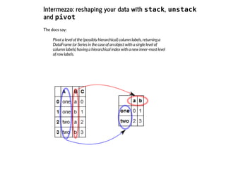
58. I
n
[
1
2
5
]
: r
e
s
u
l
t = d
f
[
'
C
'
]
.
u
n
s
t
a
c
k
(
)
r
e
s
u
l
t
O
u
t
[
1
2
5
]
: B a b
A
one 0 1
two 2 3
I
n
[
1
2
7
]
: d
f = r
e
s
u
l
t
.
s
t
a
c
k
(
)
.
r
e
s
e
t
_
i
n
d
e
x
(
n
a
m
e
=
'
C
'
)
d
f
O
u
t
[
1
2
7
]
: A B C
0 one a 0
1 one b 1
2 two a 2
3 two b 3

59. p
i
v
o
t
is similar to u
n
s
t
a
c
k
, but let you specify column names:
I
n
[
6
3
]
: d
f
.
p
i
v
o
t
(
i
n
d
e
x
=
'
A
'
, c
o
l
u
m
n
s
=
'
B
'
, v
a
l
u
e
s
=
'
C
'
)
O
u
t
[
6
3
]
: B a b
A
one 0 1
two 2 3

60. p
i
v
o
t
_
t
a
b
l
e
is similar as p
i
v
o
t
, but can work with duplicate indices and let you specify an
aggregation function:
I
n
[
1
3
0
]
: d
f = p
d
.
D
a
t
a
F
r
a
m
e
(
{
'
A
'
:
[
'
o
n
e
'
, '
o
n
e
'
, '
t
w
o
'
, '
t
w
o
'
, '
o
n
e
'
, '
t
w
o
'
]
, '
B
'
:
[
'
a
'
, '
b
'
,
'
a
'
, '
b
'
, '
a
'
, '
b
'
]
, '
C
'
:
r
a
n
g
e
(
6
)
}
)
d
f
O
u
t
[
1
3
0
]
: A B C
0 one a 0
1 one b 1
2 two a 2
3 two b 3
4 one a 4
5 two b 5
I
n
[
1
3
2
]
: d
f
.
p
i
v
o
t
_
t
a
b
l
e
(
i
n
d
e
x
=
'
A
'
, c
o
l
u
m
n
s
=
'
B
'
, v
a
l
u
e
s
=
'
C
'
, a
g
g
f
u
n
c
=
'
c
o
u
n
t
'
) #
'
m
e
a
n
'
O
u
t
[
1
3
2
]
: B a b
A
one 4 1
two 2 8

61. Back to our case study
We can now use s
t
a
c
k
to create a timeseries:
I
n
[
1
3
8
]
: d
a
t
a = d
a
t
a
.
s
e
t
_
i
n
d
e
x
(
'
d
a
t
e
'
)
I
n
[
1
3
9
]
: d
a
t
a
_
s
t
a
c
k
e
d = d
a
t
a
.
s
t
a
c
k
(
)
I
n
[
6
8
]
: d
a
t
a
_
s
t
a
c
k
e
d
O
u
t
[
6
8
]
: d
a
t
e
1
9
9
0
-
0
1
-
0
2 0
9 4
8
.
0
1
2 4
8
.
0
1
3 5
0
.
0
1
4 5
5
.
0
.
.
.
2
0
1
2
-
1
2
-
3
1 2
0 1
6
.
5
2
1 1
4
.
5
2
2 1
6
.
5
2
3 1
5
.
0
d
t
y
p
e
: f
l
o
a
t
6
4

62. Now, lets combine the two levels of the index:
I
n
[
6
9
]
: d
a
t
a
_
s
t
a
c
k
e
d = d
a
t
a
_
s
t
a
c
k
e
d
.
r
e
s
e
t
_
i
n
d
e
x
(
n
a
m
e
=
'
B
E
T
R
8
0
1
'
)
I
n
[
7
0
]
: d
a
t
a
_
s
t
a
c
k
e
d
.
i
n
d
e
x = p
d
.
t
o
_
d
a
t
e
t
i
m
e
(
d
a
t
a
_
s
t
a
c
k
e
d
[
'
d
a
t
e
'
] + d
a
t
a
_
s
t
a
c
k
e
d
[
'
l
e
v
e
l
_
1
'
]
,
f
o
r
m
a
t
=
"
%
Y
-
%
m
-
%
d
%
H
"
)
I
n
[
7
1
]
: d
a
t
a
_
s
t
a
c
k
e
d = d
a
t
a
_
s
t
a
c
k
e
d
.
d
r
o
p
(
[
'
d
a
t
e
'
, '
l
e
v
e
l
_
1
'
]
, a
x
i
s
=
1
)
I
n
[
7
2
]
: d
a
t
a
_
s
t
a
c
k
e
d
O
u
t
[
7
2
]
: BETR801
1990-01-02 09:00:00 48.0
1990-01-02 12:00:00 48.0
1990-01-02 13:00:00 50.0
1990-01-02 14:00:00 55.0
... ...
2012-12-31 20:00:00 16.5
2012-12-31 21:00:00 14.5
2012-12-31 22:00:00 16.5
2012-12-31 23:00:00 15.0
170794 rows × 1 columns

63. For this talk, I put the above code in a separate function, and repeated this for some different
monitoring stations:
I
n
[
7
3
]
: i
m
p
o
r
t a
i
r
b
a
s
e
n
o
2 = a
i
r
b
a
s
e
.
l
o
a
d
_
d
a
t
a
(
)
FR04037 (PARIS 13eme): urban background site at Square de Choisy
FR04012 (Paris, Place Victor Basch): urban traffic site at Rue d'Alesia
BETR802: urban traffic site in Antwerp, Belgium
BETN029: rural background site in Houtem, Belgium
See http://www.eea.europa.eu/themes/air/interactive/no2
(http://www.eea.europa.eu/themes/air/interactive/no2)

64. Exploring the data

65. Some useful methods:
h
e
a
d
and t
a
i
l
I
n
[
1
4
0
]
: n
o
2
.
h
e
a
d
(
3
)
O
u
t
[
1
4
0
]
: BETR801 BETN029 FR04037 FR04012
1990-01-01 00:00:00 NaN 16 NaN NaN
1990-01-01 01:00:00 NaN 18 NaN NaN
1990-01-01 02:00:00 NaN 21 NaN NaN
I
n
[
7
5
]
: n
o
2
.
t
a
i
l
(
)
O
u
t
[
7
5
]
: BETR801 BETN029 FR04037 FR04012
2012-12-31 19:00:00 21.0 2.5 28 67
2012-12-31 20:00:00 16.5 2.0 16 47
2012-12-31 21:00:00 14.5 2.5 13 43
2012-12-31 22:00:00 16.5 3.5 14 42
2012-12-31 23:00:00 15.0 3.0 13 49

66. i
n
f
o
(
)
I
n
[
7
6
]
: n
o
2
.
i
n
f
o
(
)
<
c
l
a
s
s '
p
a
n
d
a
s
.
c
o
r
e
.
f
r
a
m
e
.
D
a
t
a
F
r
a
m
e
'
>
D
a
t
e
t
i
m
e
I
n
d
e
x
: 1
9
8
8
9
5 e
n
t
r
i
e
s
, 1
9
9
0
-
0
1
-
0
1 0
0
:
0
0
:
0
0 t
o 2
0
1
2
-
1
2
-
3
1 2
3
:
0
0
:
0
0
D
a
t
a c
o
l
u
m
n
s (
t
o
t
a
l 4 c
o
l
u
m
n
s
)
:
B
E
T
R
8
0
1 1
7
0
7
9
4 n
o
n
-
n
u
l
l f
l
o
a
t
6
4
B
E
T
N
0
2
9 1
7
4
8
0
7 n
o
n
-
n
u
l
l f
l
o
a
t
6
4
F
R
0
4
0
3
7 1
2
0
3
8
4 n
o
n
-
n
u
l
l f
l
o
a
t
6
4
F
R
0
4
0
1
2 1
1
9
4
4
8 n
o
n
-
n
u
l
l f
l
o
a
t
6
4
d
t
y
p
e
s
: f
l
o
a
t
6
4
(
4
)
m
e
m
o
r
y u
s
a
g
e
: 7
.
6 M
B

67. Getting some basic summary statistics about the data with d
e
s
c
r
i
b
e
:
I
n
[
7
7
]
: n
o
2
.
d
e
s
c
r
i
b
e
(
)
O
u
t
[
7
7
]
: BETR801 BETN029 FR04037 FR04012
count 170794.000000 174807.000000 120384.000000 119448.000000
mean 47.914561 16.687756 40.040005 87.993261
std 22.230921 13.106549 23.024347 41.317684
min 0.000000 0.000000 0.000000 0.000000
25% 32.000000 7.000000 23.000000 61.000000
50% 46.000000 12.000000 37.000000 88.000000
75% 61.000000 23.000000 54.000000 115.000000
max 339.000000 115.000000 256.000000 358.000000

68. Quickly visualizing the data
I
n
[
7
8
]
: n
o
2
.
p
l
o
t
(
k
i
n
d
=
'
b
o
x
'
, y
l
i
m
=
[
0
,
2
5
0
]
)
O
u
t
[
7
8
]
: <
m
a
t
p
l
o
t
l
i
b
.
a
x
e
s
.
_
s
u
b
p
l
o
t
s
.
A
x
e
s
S
u
b
p
l
o
t a
t 0
x
a
8
3
1
8
8
4
c
>

69. I
n
[
7
9
]
: n
o
2
[
'
B
E
T
R
8
0
1
'
]
.
p
l
o
t
(
k
i
n
d
=
'
h
i
s
t
'
, b
i
n
s
=
5
0
)
O
u
t
[
7
9
]
: <
m
a
t
p
l
o
t
l
i
b
.
a
x
e
s
.
_
s
u
b
p
l
o
t
s
.
A
x
e
s
S
u
b
p
l
o
t a
t 0
x
a
8
2
f
6
5
8
c
>

70. I
n
[
8
0
]
: n
o
2
.
p
l
o
t
(
f
i
g
s
i
z
e
=
(
1
2
,
6
)
)
O
u
t
[
8
0
]
: <
m
a
t
p
l
o
t
l
i
b
.
a
x
e
s
.
_
s
u
b
p
l
o
t
s
.
A
x
e
s
S
u
b
p
l
o
t a
t 0
x
a
9
f
9
7
3
a
c
>
This does not say too much ..

71. We can select part of the data (eg the latest 500 data points):
I
n
[
8
1
]
: n
o
2
[
-
5
0
0
:
]
.
p
l
o
t
(
f
i
g
s
i
z
e
=
(
1
2
,
6
)
)
O
u
t
[
8
1
]
: <
m
a
t
p
l
o
t
l
i
b
.
a
x
e
s
.
_
s
u
b
p
l
o
t
s
.
A
x
e
s
S
u
b
p
l
o
t a
t 0
x
a
7
7
1
b
1
0
c
>
Or we can use some more advanced time series features -> next section!

72. Working with time series data
When we ensure the DataFrame has a D
a
t
e
t
i
m
e
I
n
d
e
x
, time-series related functionality
becomes available:
I
n
[
8
2
]
: n
o
2
.
i
n
d
e
x
O
u
t
[
8
2
]
: <
c
l
a
s
s '
p
a
n
d
a
s
.
t
s
e
r
i
e
s
.
i
n
d
e
x
.
D
a
t
e
t
i
m
e
I
n
d
e
x
'
>
[
1
9
9
0
-
0
1
-
0
1 0
0
:
0
0
:
0
0
, .
.
.
, 2
0
1
2
-
1
2
-
3
1 2
3
:
0
0
:
0
0
]
L
e
n
g
t
h
: 1
9
8
8
9
5
, F
r
e
q
: N
o
n
e
, T
i
m
e
z
o
n
e
: N
o
n
e

73. Indexing a time series works with strings:
I
n
[
8
3
]
: n
o
2
[
"
2
0
1
0
-
0
1
-
0
1 0
9
:
0
0
"
: "
2
0
1
0
-
0
1
-
0
1 1
2
:
0
0
"
]
O
u
t
[
8
3
]
: BETR801 BETN029 FR04037 FR04012
2010-01-01 09:00:00 17 7 19 41
2010-01-01 10:00:00 18 5 21 48
2010-01-01 11:00:00 17 4 23 63
2010-01-01 12:00:00 18 4 22 57

74. A nice feature is "partial string" indexing, where we can do implicit slicing by providing a partial
datetime string.
E.g. all data of 2012:
I
n
[
8
4
]
: n
o
2
[
'
2
0
1
2
'
]
O
u
t
[
8
4
]
: BETR801 BETN029 FR04037 FR04012
2012-01-01 00:00:00 21.0 1.0 17 56
2012-01-01 01:00:00 18.0 1.0 16 50
2012-01-01 02:00:00 20.0 1.0 14 46
2012-01-01 03:00:00 16.0 1.0 17 47
... ... ... ... ...
2012-12-31 20:00:00 16.5 2.0 16 47
2012-12-31 21:00:00 14.5 2.5 13 43
2012-12-31 22:00:00 16.5 3.5 14 42
2012-12-31 23:00:00 15.0 3.0 13 49
8784 rows × 4 columns
Or all data of January up to March 2012:

75. Time and date components can be accessed from the index:
I
n
[
1
4
5
]
: n
o
2
.
i
n
d
e
x
.
h
o
u
r
O
u
t
[
1
4
5
]
: a
r
r
a
y
(
[ 0
, 1
, 2
, .
.
.
, 2
1
, 2
2
, 2
3
]
)
I
n
[
8
7
]
: n
o
2
.
i
n
d
e
x
.
y
e
a
r
O
u
t
[
8
7
]
: a
r
r
a
y
(
[
1
9
9
0
, 1
9
9
0
, 1
9
9
0
, .
.
.
, 2
0
1
2
, 2
0
1
2
, 2
0
1
2
]
)

76. The power of pandas: r
e
s
a
m
p
l
e
A very powerfull method is r
e
s
a
m
p
l
e
: converting the frequency of the time series (e.g. from
hourly to daily data).
The time series has a frequency of 1 hour. I want to change this to daily:
I
n
[
8
8
]
: n
o
2
.
r
e
s
a
m
p
l
e
(
'
D
'
)
.
h
e
a
d
(
)
O
u
t
[
8
8
]
: BETR801 BETN029 FR04037 FR04012
1990-01-01 NaN 21.500000 NaN NaN
1990-01-02 53.923077 35.000000 NaN NaN
1990-01-03 63.000000 29.136364 NaN NaN
1990-01-04 65.250000 42.681818 NaN NaN
1990-01-05 63.846154 40.136364 NaN NaN

77. By default, r
e
s
a
m
p
l
e
takes the mean as aggregation function, but other methods can also be
specified:
I
n
[
9
0
]
: n
o
2
.
r
e
s
a
m
p
l
e
(
'
D
'
, h
o
w
=
'
m
a
x
'
)
.
h
e
a
d
(
)
O
u
t
[
9
0
]
: BETR801 BETN029 FR04037 FR04012
1990-01-01 NaN 41 NaN NaN
1990-01-02 59 59 NaN NaN
1990-01-03 103 47 NaN NaN
1990-01-04 74 58 NaN NaN
1990-01-05 84 67 NaN NaN

78. Further exploring the data:
I
n
[
1
5
2
]
: n
o
2
.
r
e
s
a
m
p
l
e
(
'
M
'
)
.
p
l
o
t
(
) # '
A
'
O
u
t
[
1
5
2
]
: <
m
a
t
p
l
o
t
l
i
b
.
a
x
e
s
.
_
s
u
b
p
l
o
t
s
.
A
x
e
s
S
u
b
p
l
o
t a
t 0
x
a
8
b
c
4
b
8
c
>
I
n
[
]
: # n
o
2
[
'
2
0
1
2
'
]
.
r
e
s
a
m
p
l
e
(
'
D
'
)
.
p
l
o
t
(
)

79. I
n
[
9
2
]
: n
o
2
.
l
o
c
[
'
2
0
0
9
'
:
, '
F
R
0
4
0
3
7
'
]
.
r
e
s
a
m
p
l
e
(
'
M
'
, h
o
w
=
[
'
m
e
a
n
'
, '
m
e
d
i
a
n
'
]
)
.
p
l
o
t
(
)
O
u
t
[
9
2
]
: <
m
a
t
p
l
o
t
l
i
b
.
a
x
e
s
.
_
s
u
b
p
l
o
t
s
.
A
x
e
s
S
u
b
p
l
o
t a
t 0
x
a
4
3
e
9
5
2
c
>

80. Question: The evolution of the yearly averages with, and the overall mean of all stations
I
n
[
9
3
]
: n
o
2
_
1
9
9
9 = n
o
2
[
'
1
9
9
9
'
:
]
n
o
2
_
1
9
9
9
.
r
e
s
a
m
p
l
e
(
'
A
'
)
.
p
l
o
t
(
)
n
o
2
_
1
9
9
9
.
m
e
a
n
(
a
x
i
s
=
1
)
.
r
e
s
a
m
p
l
e
(
'
A
'
)
.
p
l
o
t
(
c
o
l
o
r
=
'
k
'
, l
i
n
e
s
t
y
l
e
=
'
-
-
'
, l
i
n
e
w
i
d
t
h
=
4
)
O
u
t
[
9
3
]
: <
m
a
t
p
l
o
t
l
i
b
.
a
x
e
s
.
_
s
u
b
p
l
o
t
s
.
A
x
e
s
S
u
b
p
l
o
t a
t 0
x
a
4
e
a
6
0
4
c
>

81. Analysing the data

82. Intermezzo - the groupby operation (split-apply-
combine)
By "group by" we are referring to a process involving one or more of the following steps
Splitting the data into groups based on some criteria
Applying a function to each group independently
Combining the results into a data structure

83. The example of the image in pandas syntax:
I
n
[
9
4
]
: d
f = p
d
.
D
a
t
a
F
r
a
m
e
(
{
'
k
e
y
'
:
[
'
A
'
,
'
B
'
,
'
C
'
,
'
A
'
,
'
B
'
,
'
C
'
,
'
A
'
,
'
B
'
,
'
C
'
]
,
'
d
a
t
a
'
: [
0
, 5
, 1
0
, 5
, 1
0
, 1
5
, 1
0
, 1
5
, 2
0
]
}
)
d
f
O
u
t
[
9
4
]
: data key
0 0 A
1 5 B
2 10 C
3 5 A
... ... ...
5 15 C
6 10 A
7 15 B
8 20 C
9 rows × 2 columns

84. I
n
[
9
5
]
: d
f
.
g
r
o
u
p
b
y
(
'
k
e
y
'
)
.
a
g
g
r
e
g
a
t
e
(
'
s
u
m
'
) # n
p
.
s
u
m
O
u
t
[
9
5
]
: data
key
A 15
B 30
C 45
I
n
[
9
6
]
: d
f
.
g
r
o
u
p
b
y
(
'
k
e
y
'
)
.
s
u
m
(
)
O
u
t
[
9
6
]
: data
key
A 15
B 30
C 45

85. Back to the air quality data
Question: how does the typical monthly profile look like for the different stations?
First, we add a column to the dataframe that indicates the month (integer value of 1 to 12):
I
n
[
9
7
]
: n
o
2
[
'
m
o
n
t
h
'
] = n
o
2
.
i
n
d
e
x
.
m
o
n
t
h

86. Now, we can calculate the mean of each month over the different years:
I
n
[
9
8
]
: n
o
2
.
g
r
o
u
p
b
y
(
'
m
o
n
t
h
'
)
.
m
e
a
n
(
)
O
u
t
[
9
8
]
: BETR801 BETN029 FR04037 FR04012
month
1 50.927088 20.304075 47.634409 82.472813
2 54.168021 19.938929 50.564499 83.973207
3 54.598322 19.424205 47.862715 96.272138
4 51.491741 18.183433 40.943117 95.962862
... ... ... ... ...
9 49.220250 14.605979 39.706019 93.000316
10 50.894911 17.660149 44.010934 86.297836
11 50.254468 19.372193 45.564683 87.173878
12 48.644117 21.007089 45.262243 81.817977
12 rows × 4 columns

87. I
n
[
9
9
]
: n
o
2
.
g
r
o
u
p
b
y
(
'
m
o
n
t
h
'
)
.
m
e
a
n
(
)
.
p
l
o
t
(
)
O
u
t
[
9
9
]
: <
m
a
t
p
l
o
t
l
i
b
.
a
x
e
s
.
_
s
u
b
p
l
o
t
s
.
A
x
e
s
S
u
b
p
l
o
t a
t 0
x
a
9
0
1
b
0
c
c
>

88. Question: The typical diurnal profile for the different stations
I
n
[
1
5
6
]
: n
o
2
.
g
r
o
u
p
b
y
(
n
o
2
.
i
n
d
e
x
.
h
o
u
r
)
.
m
e
a
n
(
)
.
p
l
o
t
(
)
O
u
t
[
1
5
6
]
: <
m
a
t
p
l
o
t
l
i
b
.
a
x
e
s
.
_
s
u
b
p
l
o
t
s
.
A
x
e
s
S
u
b
p
l
o
t a
t 0
x
a
3
2
f
2
f
e
c
>

89. Question: What is the difference in the typical diurnal profile between week and weekend
days.
I
n
[
1
0
1
]
: n
o
2
.
i
n
d
e
x
.
w
e
e
k
d
a
y
?
I
n
[
1
0
2
]
: n
o
2
[
'
w
e
e
k
d
a
y
'
] = n
o
2
.
i
n
d
e
x
.
w
e
e
k
d
a
y

90. Add a column indicating week/weekend
I
n
[
1
0
3
]
: n
o
2
[
'
w
e
e
k
e
n
d
'
] = n
o
2
[
'
w
e
e
k
d
a
y
'
]
.
i
s
i
n
(
[
5
, 6
]
)
I
n
[
1
0
4
]
: d
a
t
a
_
w
e
e
k
e
n
d = n
o
2
.
g
r
o
u
p
b
y
(
[
'
w
e
e
k
e
n
d
'
, n
o
2
.
i
n
d
e
x
.
h
o
u
r
]
)
.
m
e
a
n
(
)
d
a
t
a
_
w
e
e
k
e
n
d
.
h
e
a
d
(
)
O
u
t
[
1
0
4
]
: BETR801 BETN029 FR04037 FR04012 month weekday
weekend
False
0 40.008066 17.487512 34.439398 52.094663 6.520355 1.998157
1 38.281875 17.162671 31.585121 44.721629 6.518121 1.997315
2 38.601189 16.800076 30.865143 43.518539 6.520511 2.000000
3 42.633946 16.591031 32.963500 51.942135 6.518038 2.002360
4 49.853566 16.791971 40.780162 72.547472 6.514098 2.003883

91. I
n
[
1
0
5
]
: d
a
t
a
_
w
e
e
k
e
n
d
_
F
R
0
4
0
1
2 = d
a
t
a
_
w
e
e
k
e
n
d
[
'
F
R
0
4
0
1
2
'
]
.
u
n
s
t
a
c
k
(
l
e
v
e
l
=
0
)
d
a
t
a
_
w
e
e
k
e
n
d
_
F
R
0
4
0
1
2
.
h
e
a
d
(
)
O
u
t
[
1
0
5
]
: weekend False True
0 52.094663 69.817219
1 44.721629 60.697248
2 43.518539 54.407904
3 51.942135 53.534933
4 72.547472 57.472830

92. I
n
[
1
0
6
]
: d
a
t
a
_
w
e
e
k
e
n
d
_
F
R
0
4
0
1
2
.
p
l
o
t
(
)
O
u
t
[
1
0
6
]
: <
m
a
t
p
l
o
t
l
i
b
.
a
x
e
s
.
_
s
u
b
p
l
o
t
s
.
A
x
e
s
S
u
b
p
l
o
t a
t 0
x
a
8
f
0
c
f
e
c
>

93. Question: What are the number of exceedances of hourly values above the European limit 200
µg/m3 ?
I
n
[
1
0
7
]
: e
x
c
e
e
d
a
n
c
e
s = n
o
2 > 2
0
0
I
n
[
1
0
8
]
: # g
r
o
u
p b
y y
e
a
r a
n
d c
o
u
n
t e
x
c
e
e
d
a
n
c
e
s (
s
u
m o
f b
o
o
l
e
a
n
)
e
x
c
e
e
d
a
n
c
e
s = e
x
c
e
e
d
a
n
c
e
s
.
g
r
o
u
p
b
y
(
e
x
c
e
e
d
a
n
c
e
s
.
i
n
d
e
x
.
y
e
a
r
)
.
s
u
m
(
)
I
n
[
1
0
9
]
: a
x = e
x
c
e
e
d
a
n
c
e
s
.
l
o
c
[
2
0
0
5
:
]
.
p
l
o
t
(
k
i
n
d
=
'
b
a
r
'
)
a
x
.
a
x
h
l
i
n
e
(
1
8
, c
o
l
o
r
=
'
k
'
, l
i
n
e
s
t
y
l
e
=
'
-
-
'
)
O
u
t
[
1
0
9
]
: <
m
a
t
p
l
o
t
l
i
b
.
l
i
n
e
s
.
L
i
n
e
2
D a
t 0
x
a
8
e
d
1
f
c
c
>

94. Question: Visualize the typical week profile for the different stations as boxplots.
Tip: the boxplot method of a DataFrame expects the data for the different boxes in different
columns)
I
n
[
1
1
0
]
: # a
d
d a w
e
e
k
d
a
y a
n
d w
e
e
k c
o
l
u
m
n
n
o
2
[
'
w
e
e
k
d
a
y
'
] = n
o
2
.
i
n
d
e
x
.
w
e
e
k
d
a
y
n
o
2
[
'
w
e
e
k
'
] = n
o
2
.
i
n
d
e
x
.
w
e
e
k
n
o
2
.
h
e
a
d
(
)
O
u
t
[
1
1
0
]
: BETR801 BETN029 FR04037 FR04012 month weekday weekend week
1990-01-
01
00:00:00
NaN 16 NaN NaN 1 0 False 1
1990-01-
01
01:00:00
NaN 18 NaN NaN 1 0 False 1
1990-01-
01
02:00:00
NaN 21 NaN NaN 1 0 False 1
1990-01-
01
03:00:00
NaN 26 NaN NaN 1 0 False 1
1990-01-
01
04:00:00
NaN 21 NaN NaN 1 0 False 1

95. I
n
[
1
1
1
]
: # p
i
v
o
t t
a
b
l
e s
o t
h
a
t t
h
e w
e
e
k
d
a
y
s a
r
e t
h
e d
i
f
f
e
r
e
n
t c
o
l
u
m
n
s
d
a
t
a
_
p
i
v
o
t
e
d = n
o
2
[
'
2
0
1
2
'
]
.
p
i
v
o
t
_
t
a
b
l
e
(
c
o
l
u
m
n
s
=
'
w
e
e
k
d
a
y
'
, i
n
d
e
x
=
'
w
e
e
k
'
, v
a
l
u
e
s
=
'
F
R
0
4
0
3
7
'
)
d
a
t
a
_
p
i
v
o
t
e
d
.
h
e
a
d
(
)
O
u
t
[
1
1
1
]
: weekday 0 1 2 3 4 5 6
week
1 24.625000 23.875000 26.208333 17.500000 40.208333 24.625000 22.375000
2 39.125000 44.125000 57.583333 50.750000 40.791667 34.750000 32.250000
3 45.208333 66.333333 51.958333 28.250000 28.291667 18.416667 18.333333
4 35.333333 49.500000 49.375000 48.916667 63.458333 34.250000 25.250000
5 47.791667 38.791667 54.333333 50.041667 51.458333 46.541667 35.458333
I
n
[
1
1
3
]
: b
o
x = d
a
t
a
_
p
i
v
o
t
e
d
.
b
o
x
p
l
o
t
(
)

96. Exercise: Calculate the correlation between the different stations
I
n
[
1
1
4
]
: n
o
2
[
[
'
B
E
T
R
8
0
1
'
, '
B
E
T
N
0
2
9
'
, '
F
R
0
4
0
3
7
'
, '
F
R
0
4
0
1
2
'
]
]
.
c
o
r
r
(
)
O
u
t
[
1
1
4
]
: BETR801 BETN029 FR04037 FR04012
BETR801 1.000000 0.464085 0.561676 0.394446
BETN029 0.464085 1.000000 0.401864 0.186997
FR04037 0.561676 0.401864 1.000000 0.433466
FR04012 0.394446 0.186997 0.433466 1.000000
I
n
[
1
1
5
]
: n
o
2
[
[
'
B
E
T
R
8
0
1
'
, '
B
E
T
N
0
2
9
'
, '
F
R
0
4
0
3
7
'
, '
F
R
0
4
0
1
2
'
]
]
.
r
e
s
a
m
p
l
e
(
'
D
'
)
.
c
o
r
r
(
)
O
u
t
[
1
1
5
]
: BETR801 BETN029 FR04037 FR04012
BETR801 1.000000 0.581701 0.663855 0.459885
BETN029 0.581701 1.000000 0.527390 0.312484
FR04037 0.663855 0.527390 1.000000 0.453584
FR04012 0.459885 0.312484 0.453584 1.000000

97. Further reading
the documentation:
Wes McKinney's book "Python for Data Analysis"
lots of tutorials on the internet, eg
http://pandas.pydata.org/pandas-docs/stable/
(http://pandas.pydata.org/pandas-docs/stable/)
http://github.com/jvns/pandas-cookbook
(http://github.com/jvns/pandas-cookbook)

98. What's new in pandas
Some recent enhancements of the last year (versions 0.14 to 0.16):
Better integration for categorical data (C
a
t
e
g
o
r
i
c
a
l
and C
a
t
e
g
o
r
i
c
a
l
I
n
d
e
x
)
The same for T
i
m
e
d
e
l
t
a
and T
i
m
e
d
e
l
t
a
I
n
d
e
x
More flexible SQL interface based on s
q
l
a
l
c
h
e
m
y
MultiIndexing using slicers
.
d
t
accessor for accesing datetime-properties from columns
Groupby enhancements
And a lot of enhancements and bug fixes

99. How can you help?
We need you!
Contributions are very welcome and can be in different domains:
reporting issues
improving the documentation
testing release candidates and provide feedback
triaging and fixing bugs
implementing new features
spreading the word
-> https://github.com/pydata/pandas (https://github.com/pydata/pandas)

100. Thanks for listening! Questions?
Slides and data: Source:
Slides presented with 'live reveal'
https://github.com/jorisvandenbossche (https://github.com/jorisvandenbossche)
@jorisvdbossche (https://twitter.com/jorisvdbossche)
https://github.com/jorisvandenbossche/2015-PyDataParis
(https://github.com/jorisvandenbossche/2015-PyDataParis)
https://github.com/damianavila/RISE
(https://github.com/damianavila/RISE)