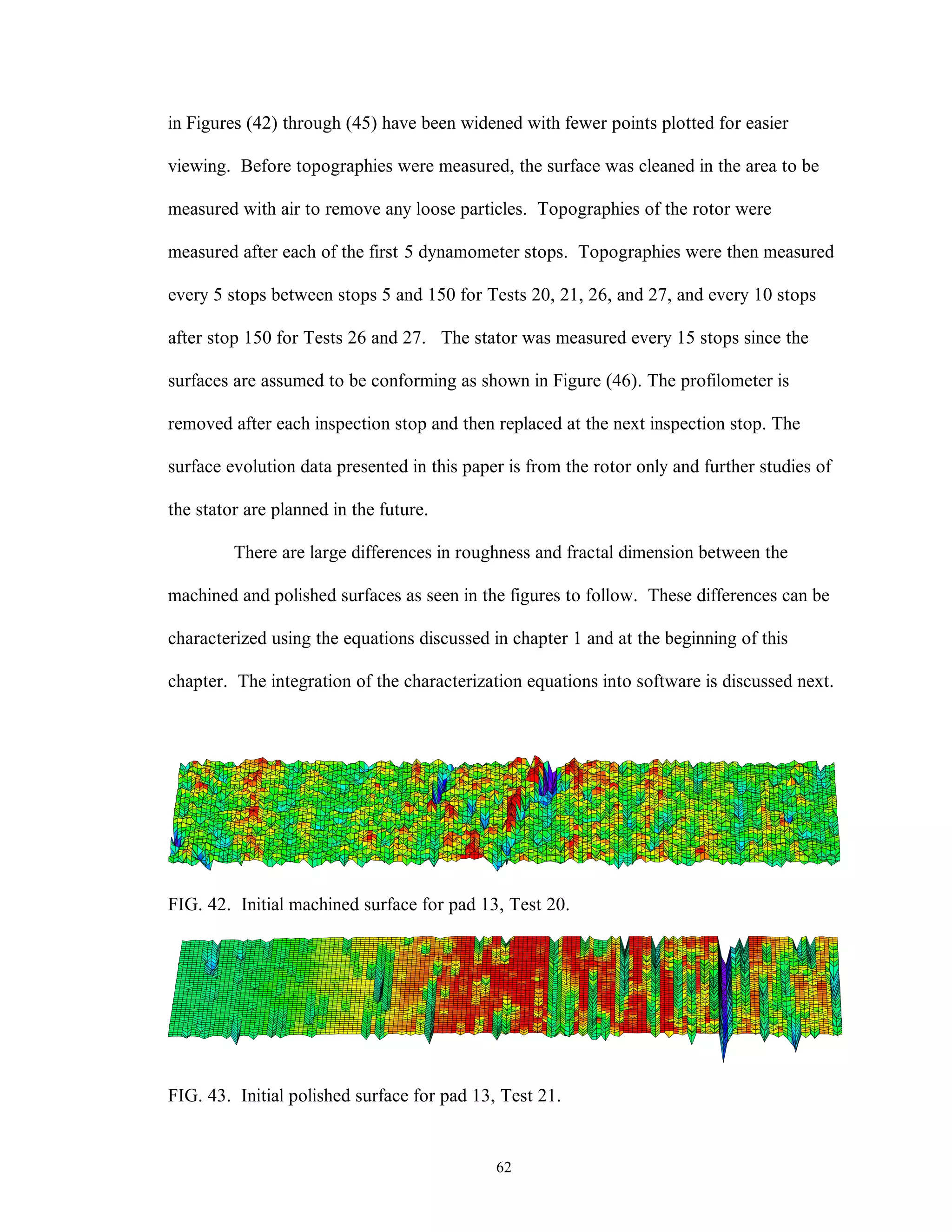
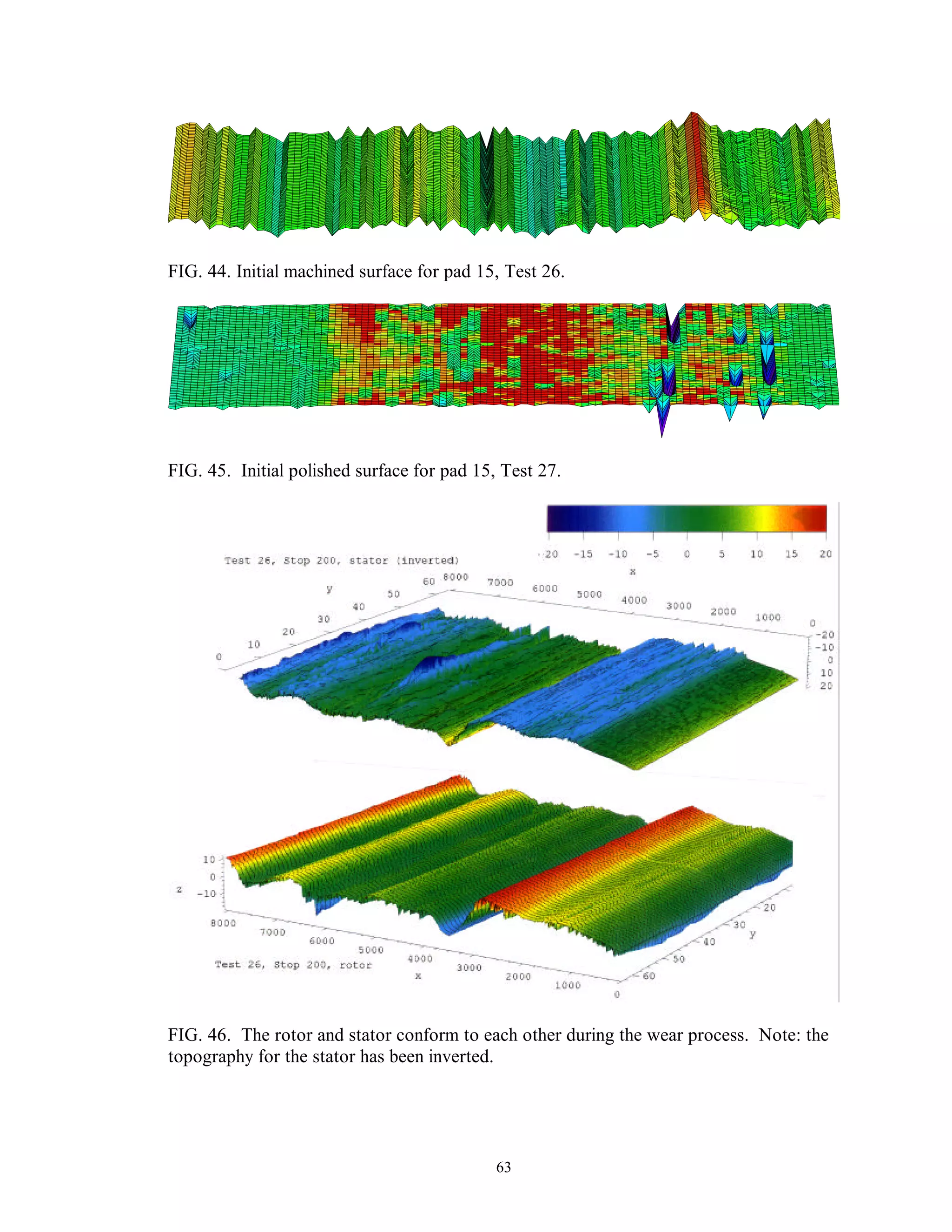
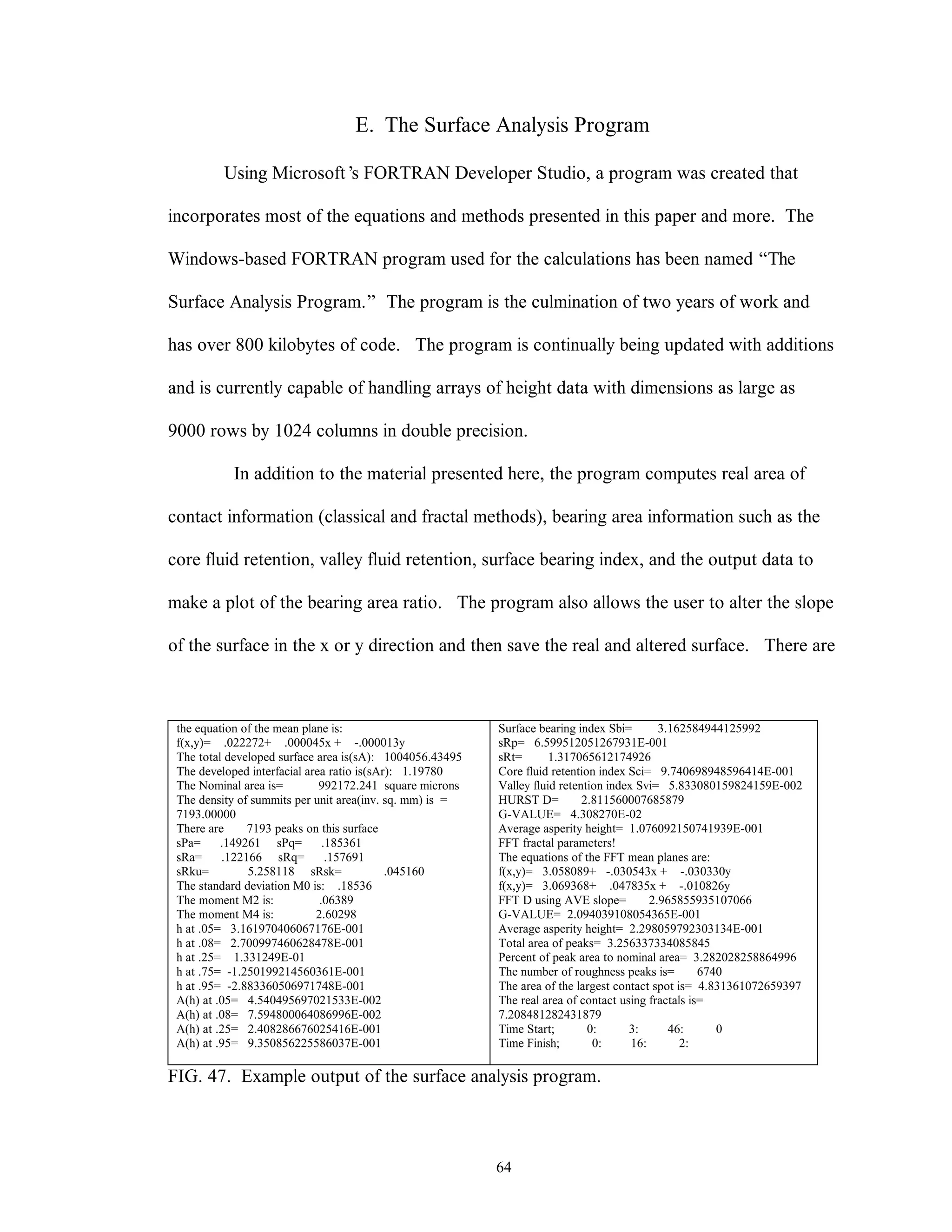
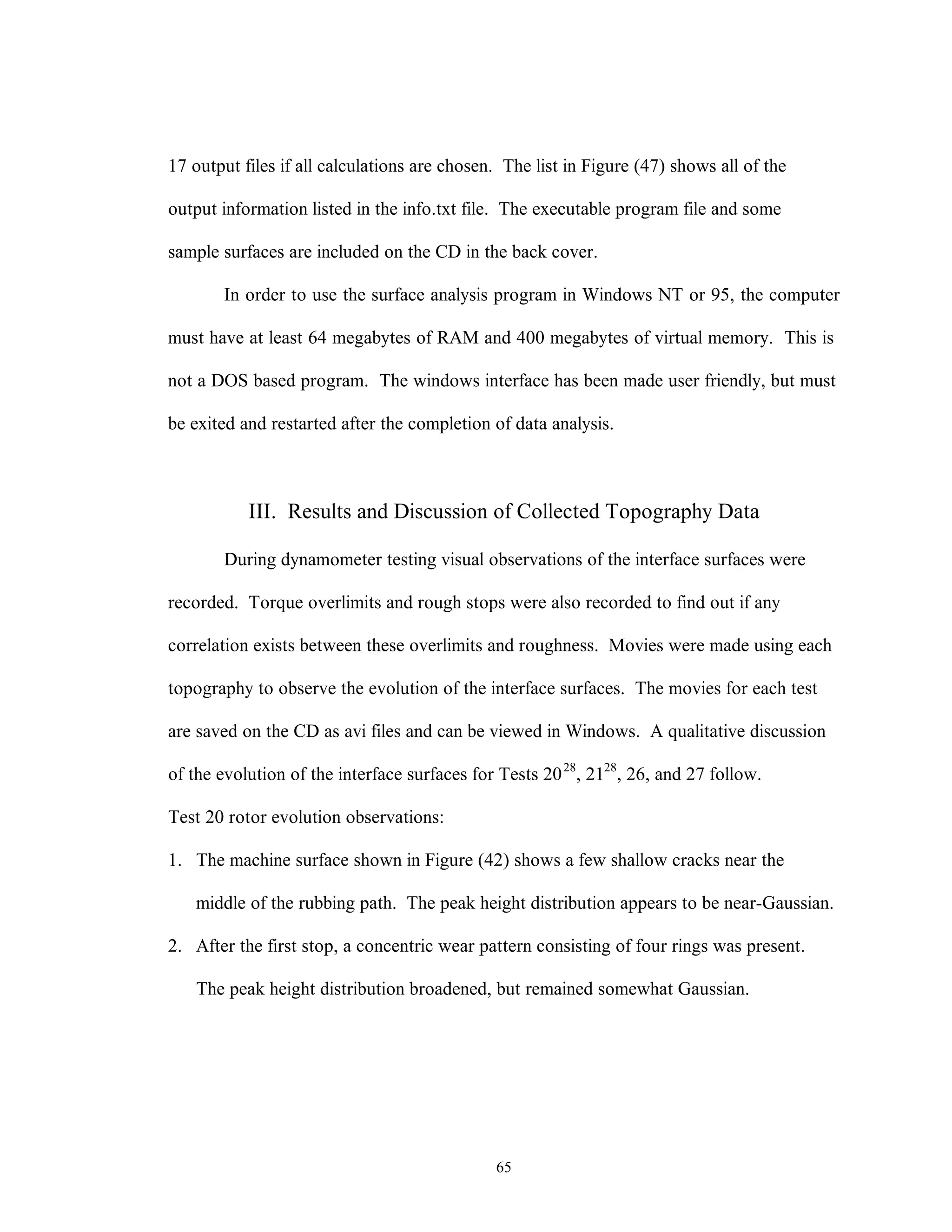
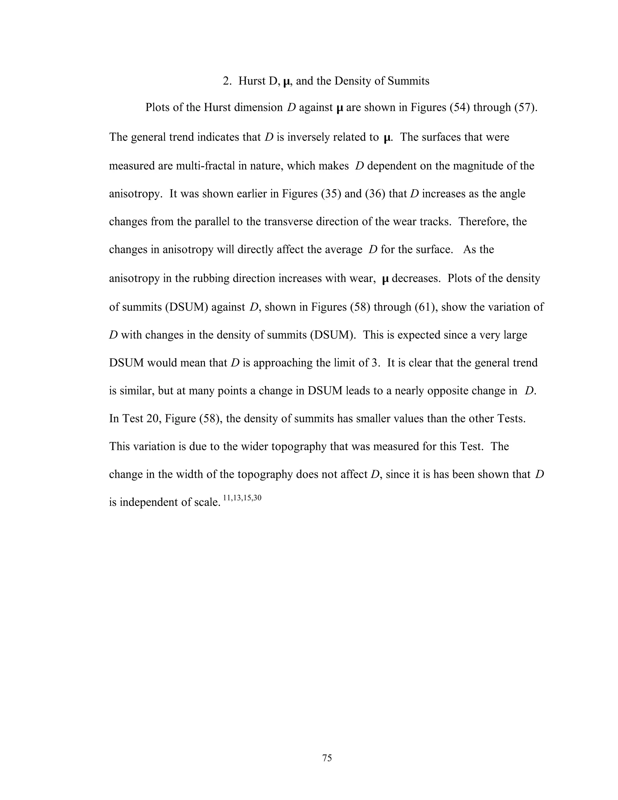
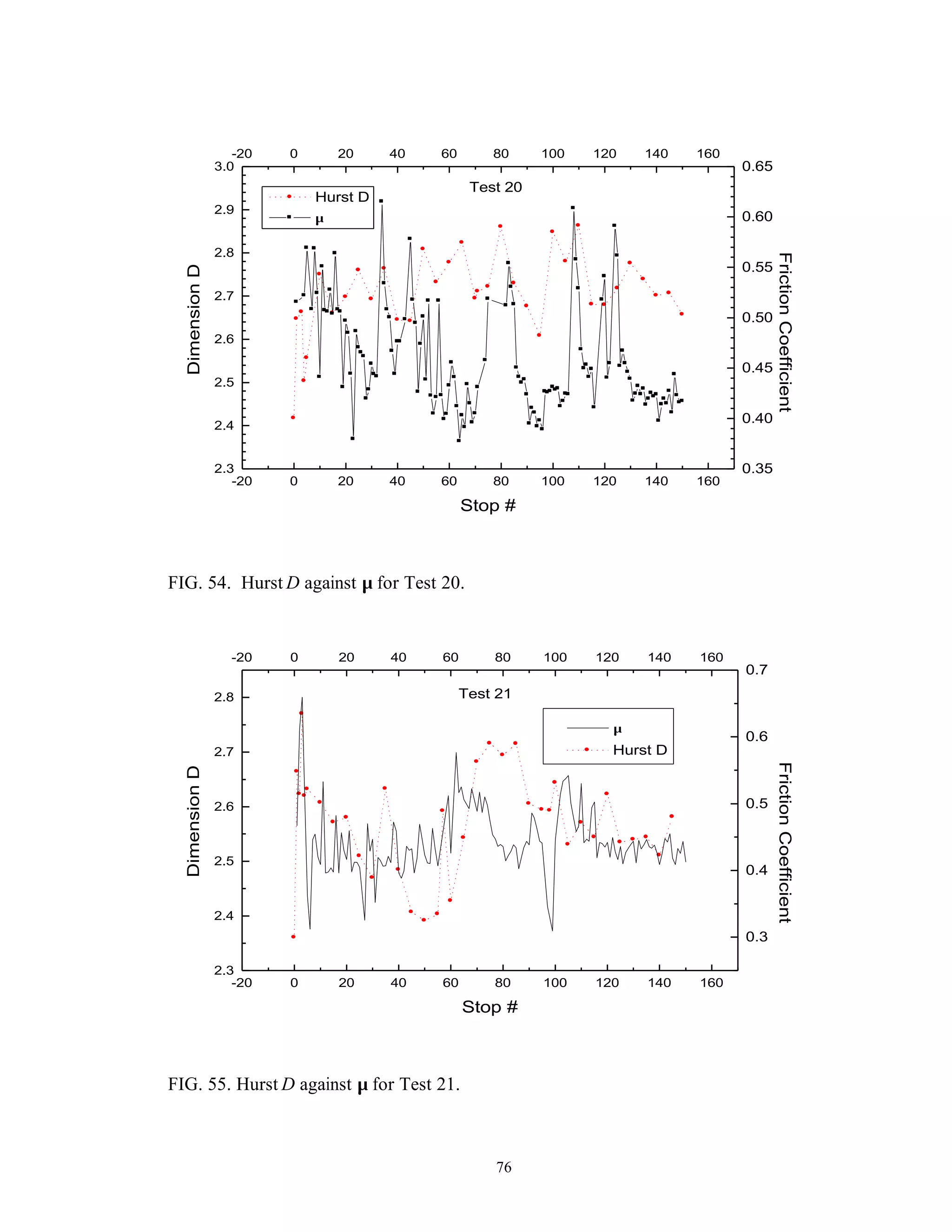
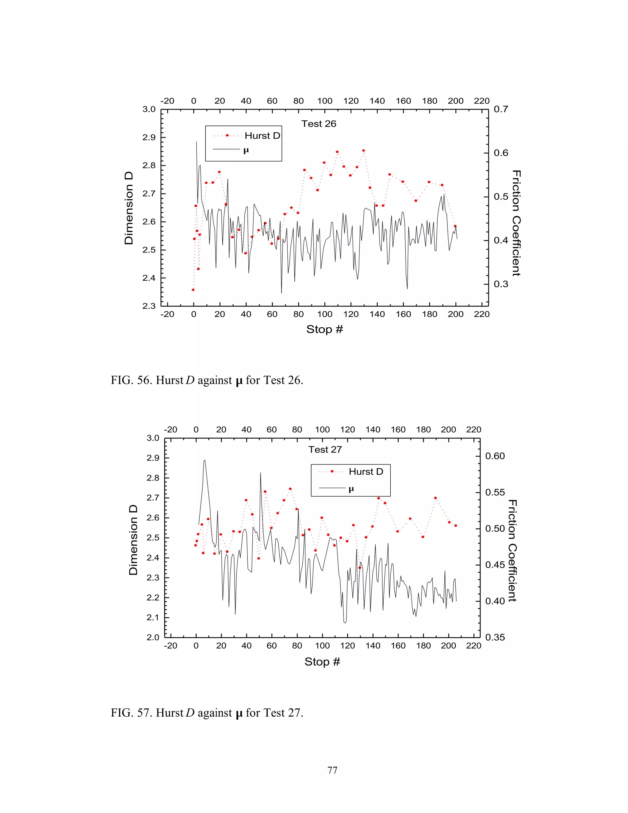
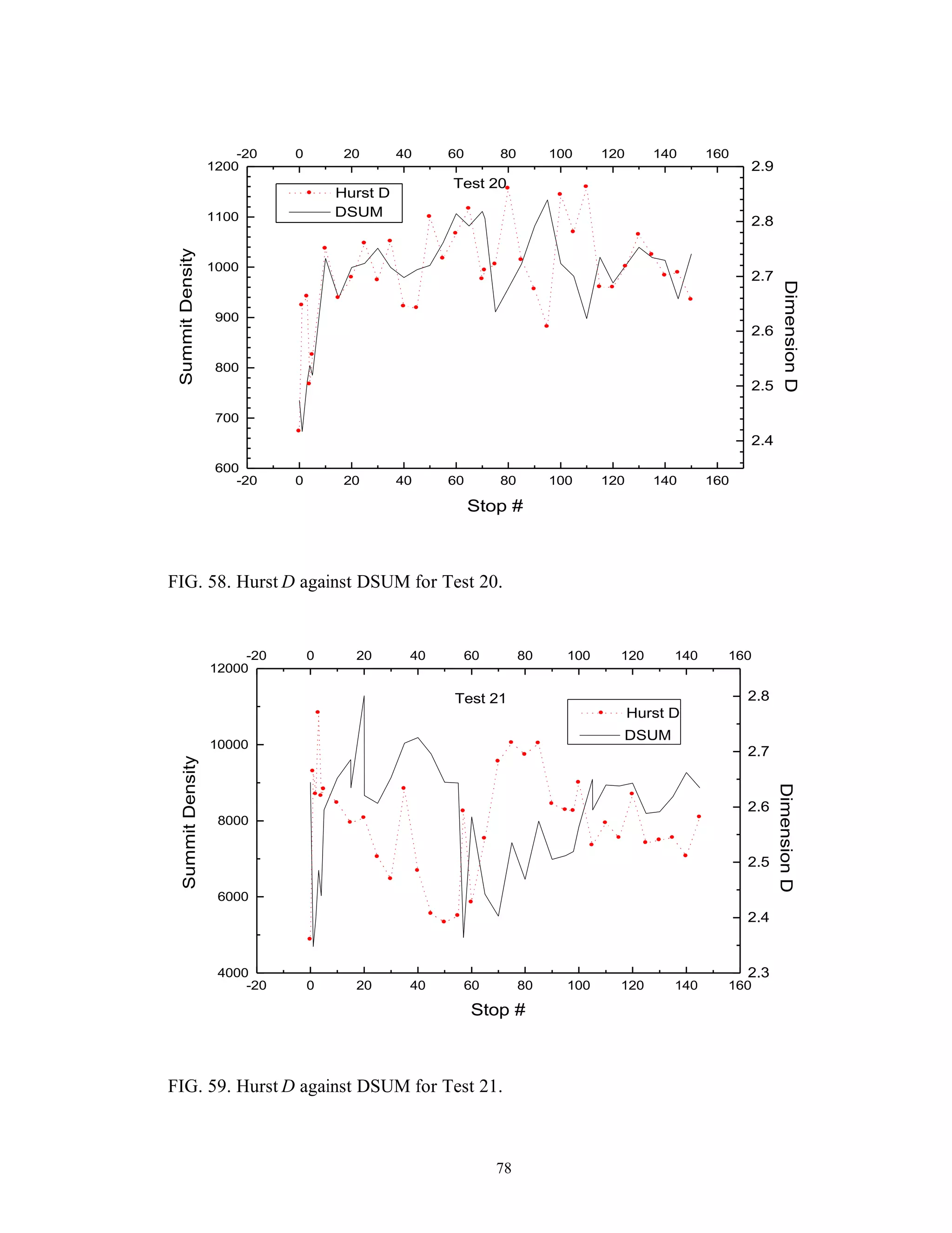
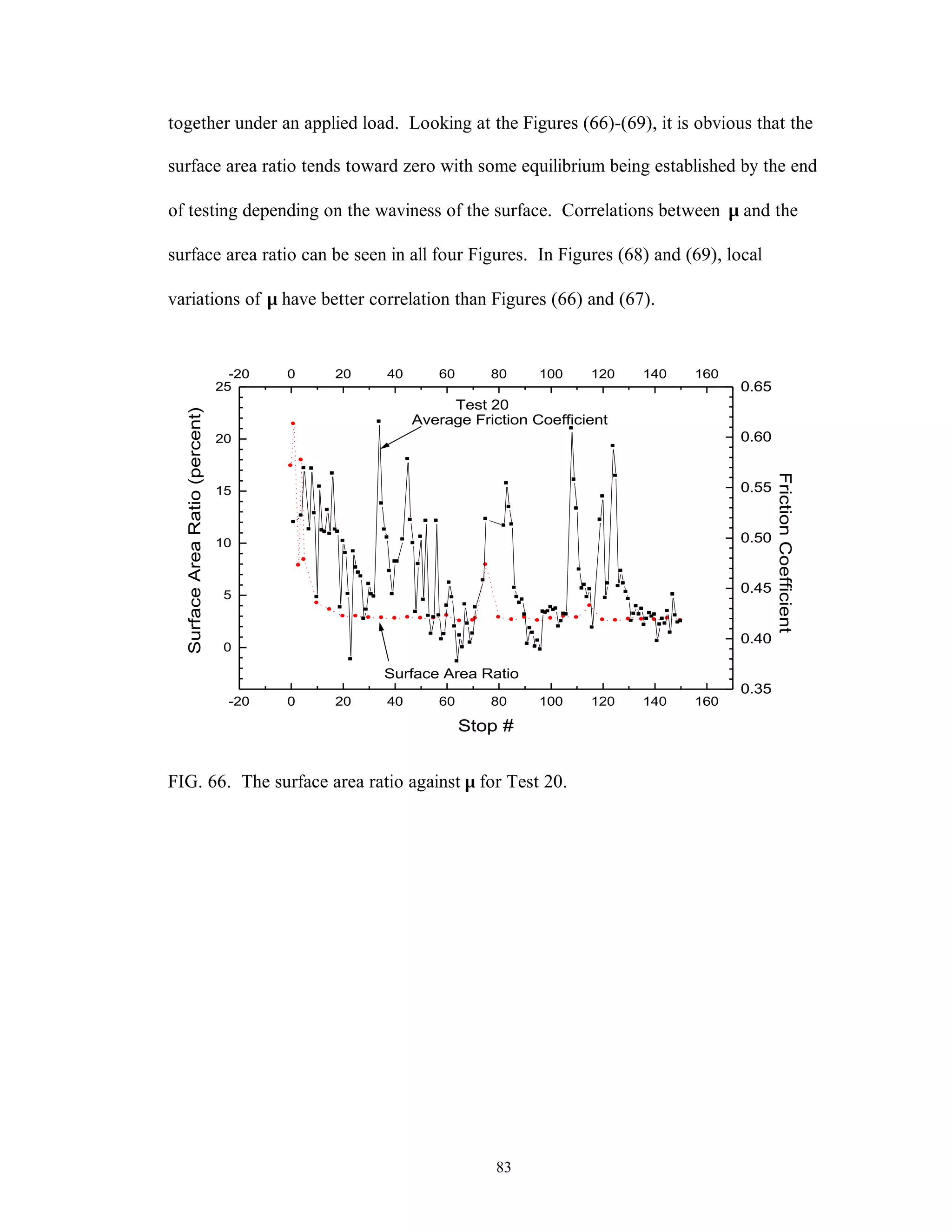
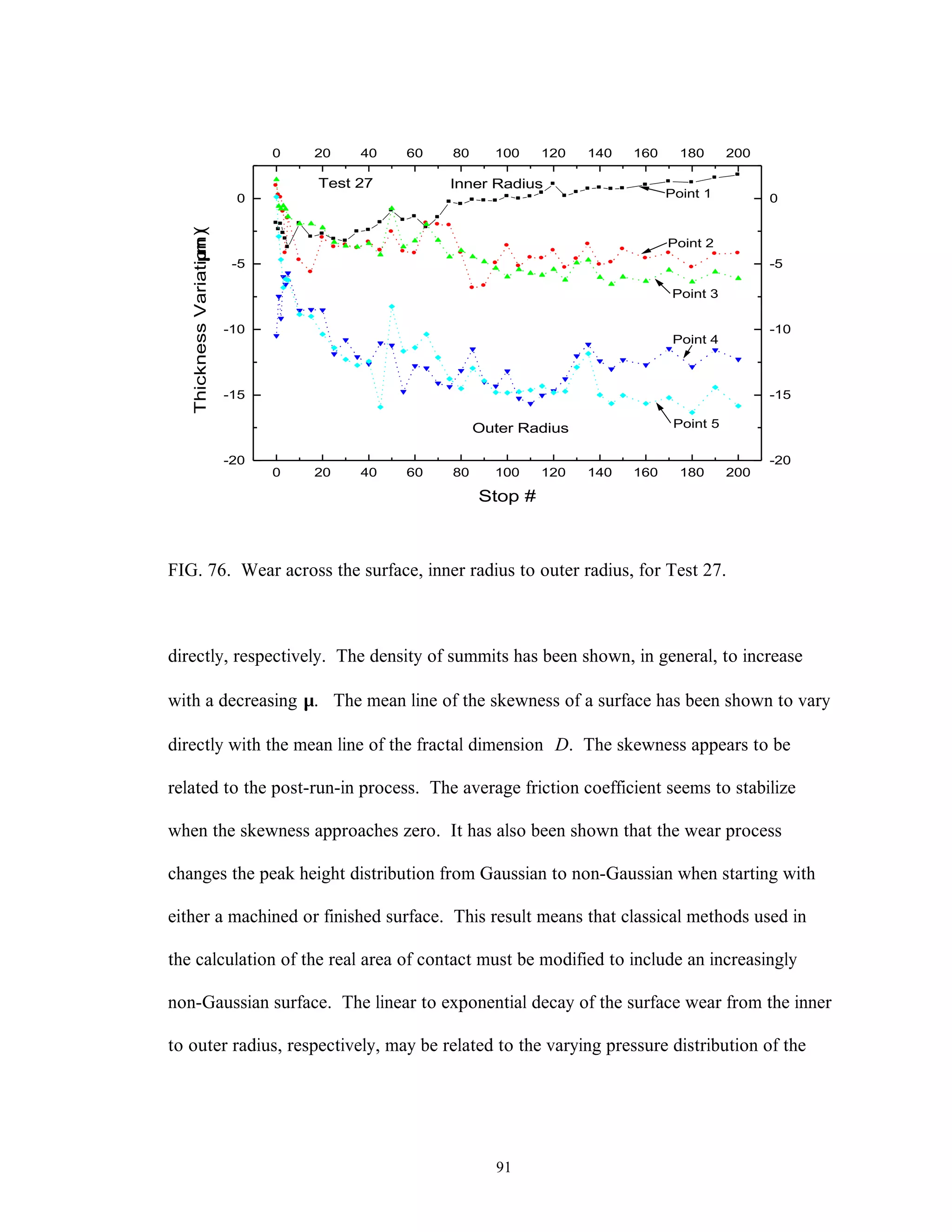
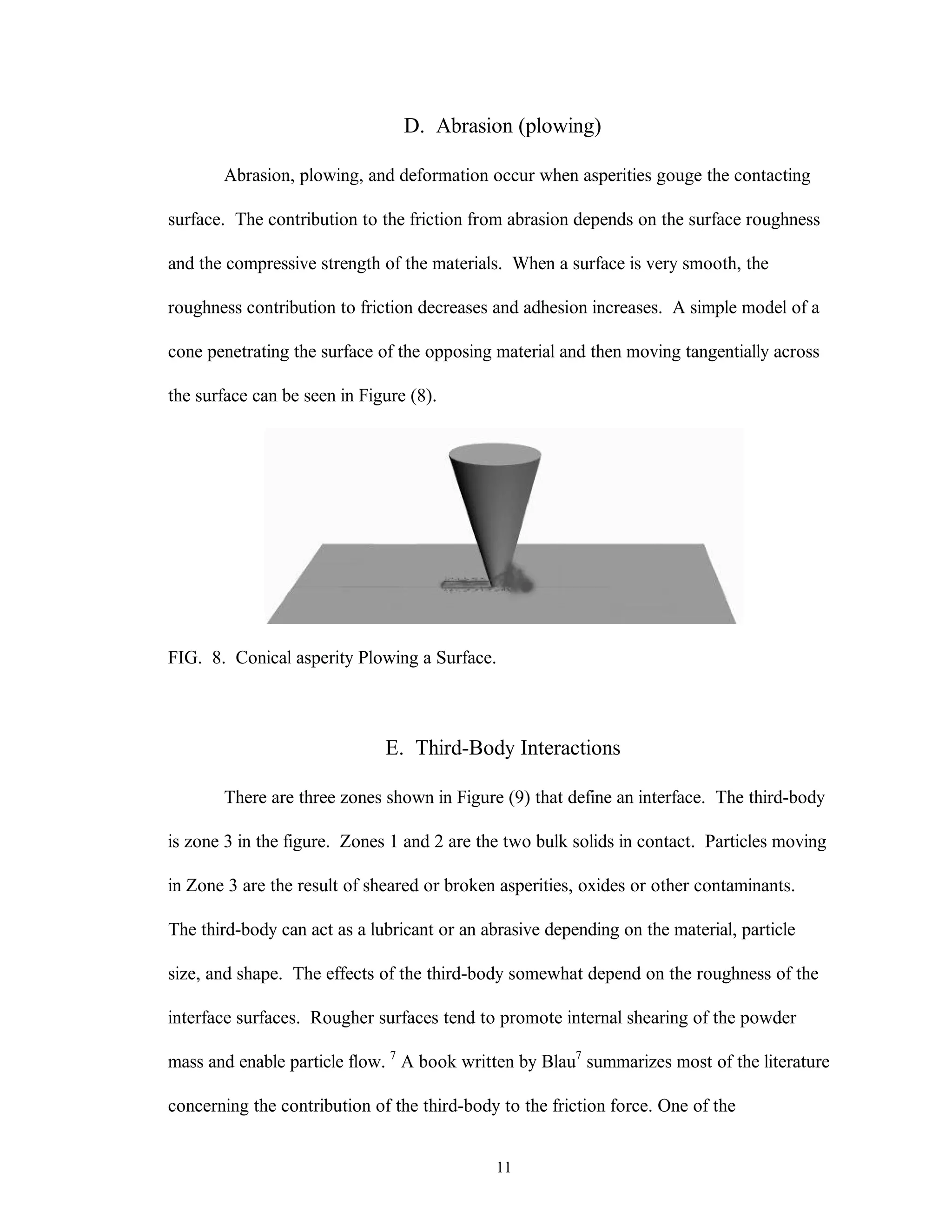
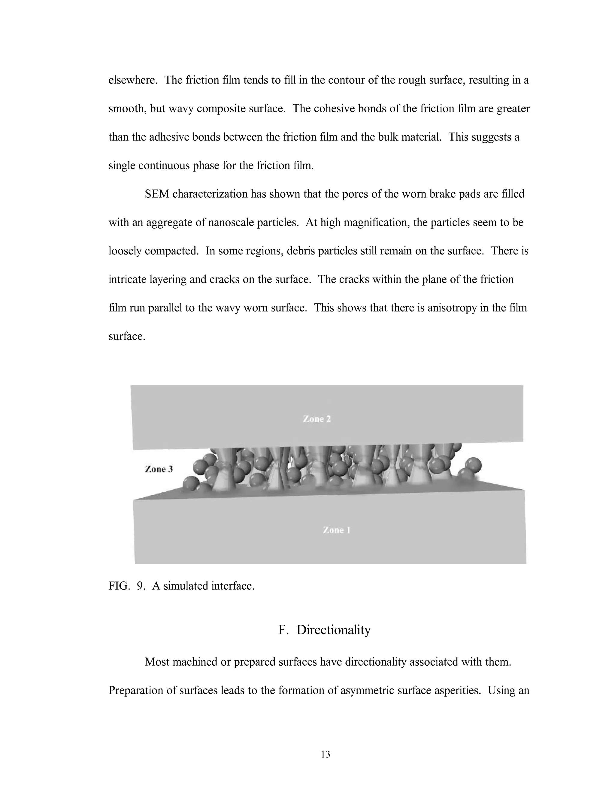
This thesis examines the surface characterization and evolution of sub-scale brake materials. Experimentation is conducted on Carbon-Carbon (C-C) composites used in aircraft brakes. Testing is performed using a dynamometer to study how the absorbed energy and friction coefficient change under varying conditions. Surface topography measurements are collected using a profilometer and analyzed using statistical and fractal geometry methods. Relationships found from the analysis include friction coefficient varying with roughness, and correlations between fractal parameters, density of summits, skewness, and friction coefficient. The study provides insight into brake material performance and evolution over multiple stops.

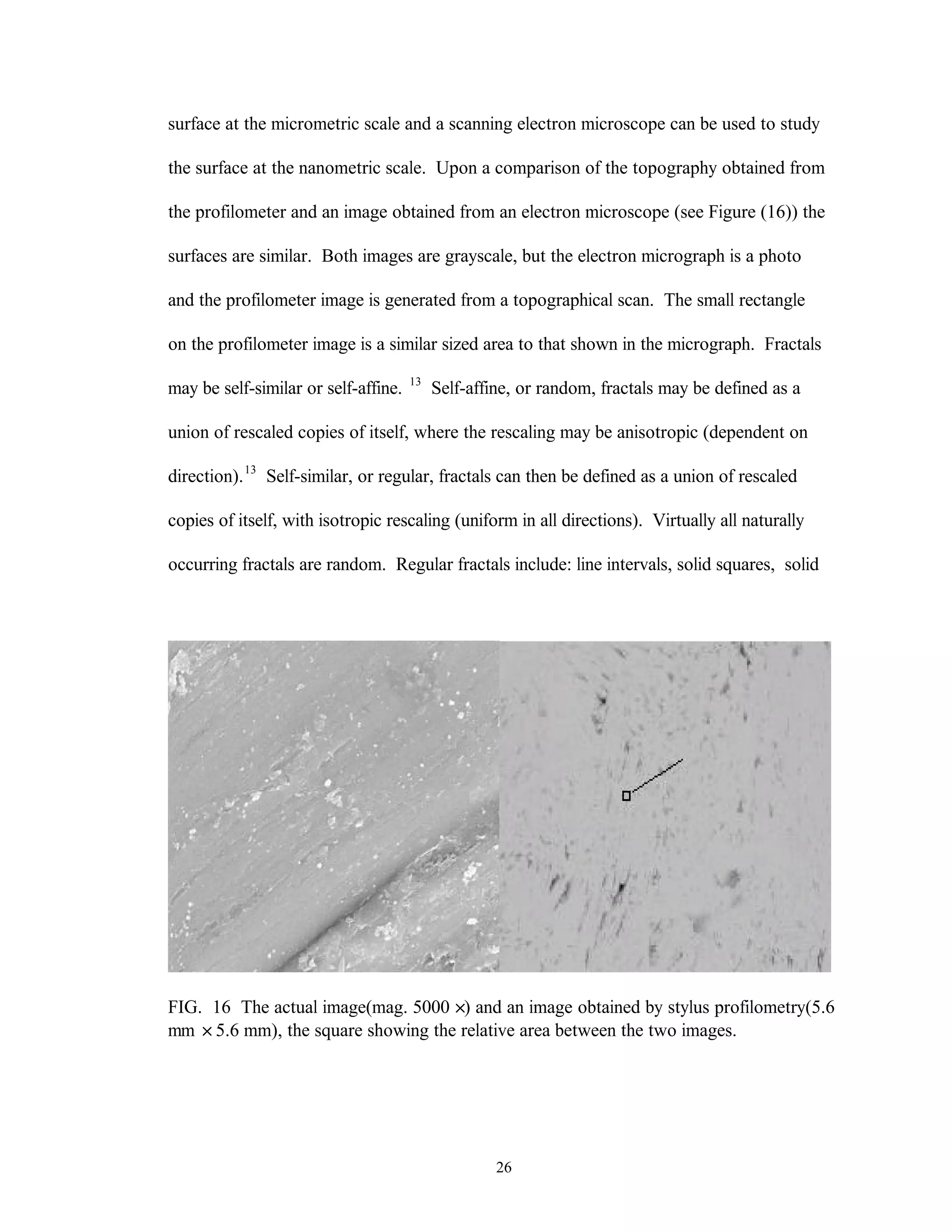
![20
where yi is the set of y values or heights associated with each xi along the measured profile
line. The roughness line is the collection of points ( xi, y yi i− ′). The number k is the
number of points averaged around each yi. λc is the roughness long wavelength cut-off
value specified by the ASME for a particular tip radius and sampling interval; and λs is
used in place of λc to determine the roughness at short wavelengths. The value of
α π= =ln / .2 04697 .9
A method of filtering not discussed in the ASME standard is adjacent averaging.
As in Gaussian filtering, adjacent averaging averages a fixed number of adjacent heights
around each specified point xi. The tip radius, the traversing length, and the number of
data points collected determine the number of adjacent points averaged. This method
produces a mean line (the waviness component) that is subtracted from the raw profile to
give the roughness component. The two components yield the original profile when
added together. The equation for adjacent averaging for each point i is
(2) ′=
+
+
−
∑y
k
yi i k
k
k
1
2 1
and the roughness line is comprised of the set of points ( xi, y yi i− ′).
Equations (1) and (2) are essentially the same with the exception that (1) contains
a weighting function. The weighting function is usually constant, but it can vary when the
sample spacing varies (phase variations). The function provides some degree of
smoothing of the real profile and compensates for possible sample spacing variations. The
amount of smoothing is based on the cutoff standards specified by ASME B46.1-1995 [2,
see section 9, table 9-2]. The cutoff standards do not apply when the surface structures to
be assessed are outside of the bandwidths 2.5 µm < λ< 0.8 mm for a 2-µm tip radius and](https://image.slidesharecdn.com/8bf0a7f6-6ca6-4e58-84b7-6c9f74012ad7-160219070136/75/TodPmastersthesis-31-2048.jpg)
![21
8 µm < λ< 2.5 mm for 5-µm tip radius or if damage occurs to the surface when using a
skidless instrument. The application of adjacent averaging requires the user to determine
the appropriate bandwidth parameter to use. In determining the bandwidth, the user must
know the number of data points taken over the tracelength. A suitable bandwidth
parameter would be 1 % of the number of data points collected over the tracelength.
Without obtaining too much fine structure, a 1 % bandwidth parameter would remove
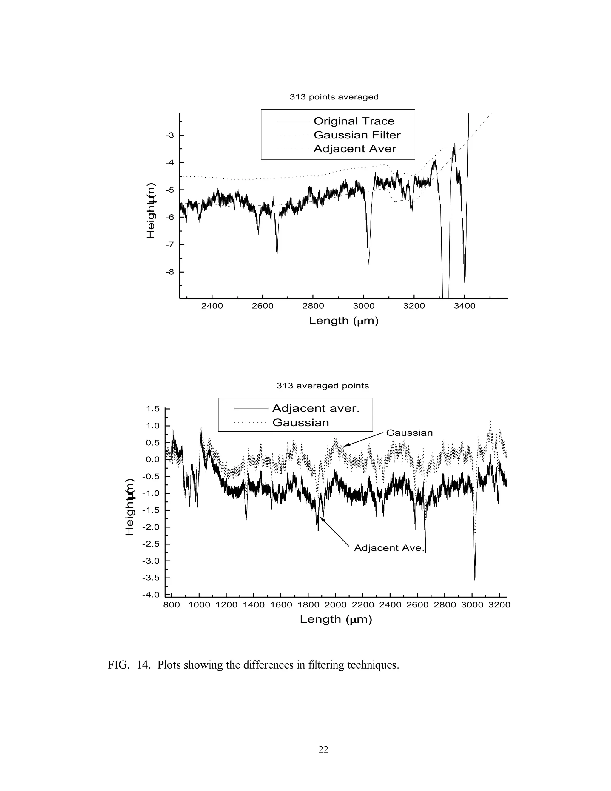
most of the waviness. Plots comparing Gaussian and adjacent averaging filter techniques
are shown in Figures (14a and b). Adjacent averaging usually results in a better mean line
through the raw data than the Gaussian filter produces.
After the data has gone through some sort of filtering process and has been
separated into roughness and waviness components, a number of statistical equations can
be used to determine roughness parameters.
A few of the more common parameters and equations are shown as equations (3)
below.
(3)
( )[ ]
( )
R
l
Y x
R
l
Y x
R
N
Z Z Z Z
R Y Y
R
n
Y
m
Y
a
x
N
q
x
N
z N
zISO Pk
k
Nk
k
c Pk
k
n
Nk
k
m
=
=
= + + + +
= +
= +
=
=
= =
= =
∑
∑
∑ ∑
∑ ∑
1
1
1
1
5
1
5
1 1
0
2
0
1
2
1 2 3
1
5
1
5
1 1
( )
.....
(arithmetical mean devi ation)
(root - mean - square deviation)
(roughness depth)
where l is the evaluation length, Y(x) is the data set, N is the number of points, and ZN is
the height from the highest to the deepest profile point within regularly spaced intervals.](https://image.slidesharecdn.com/8bf0a7f6-6ca6-4e58-84b7-6c9f74012ad7-160219070136/75/TodPmastersthesis-32-2048.jpg)
![24
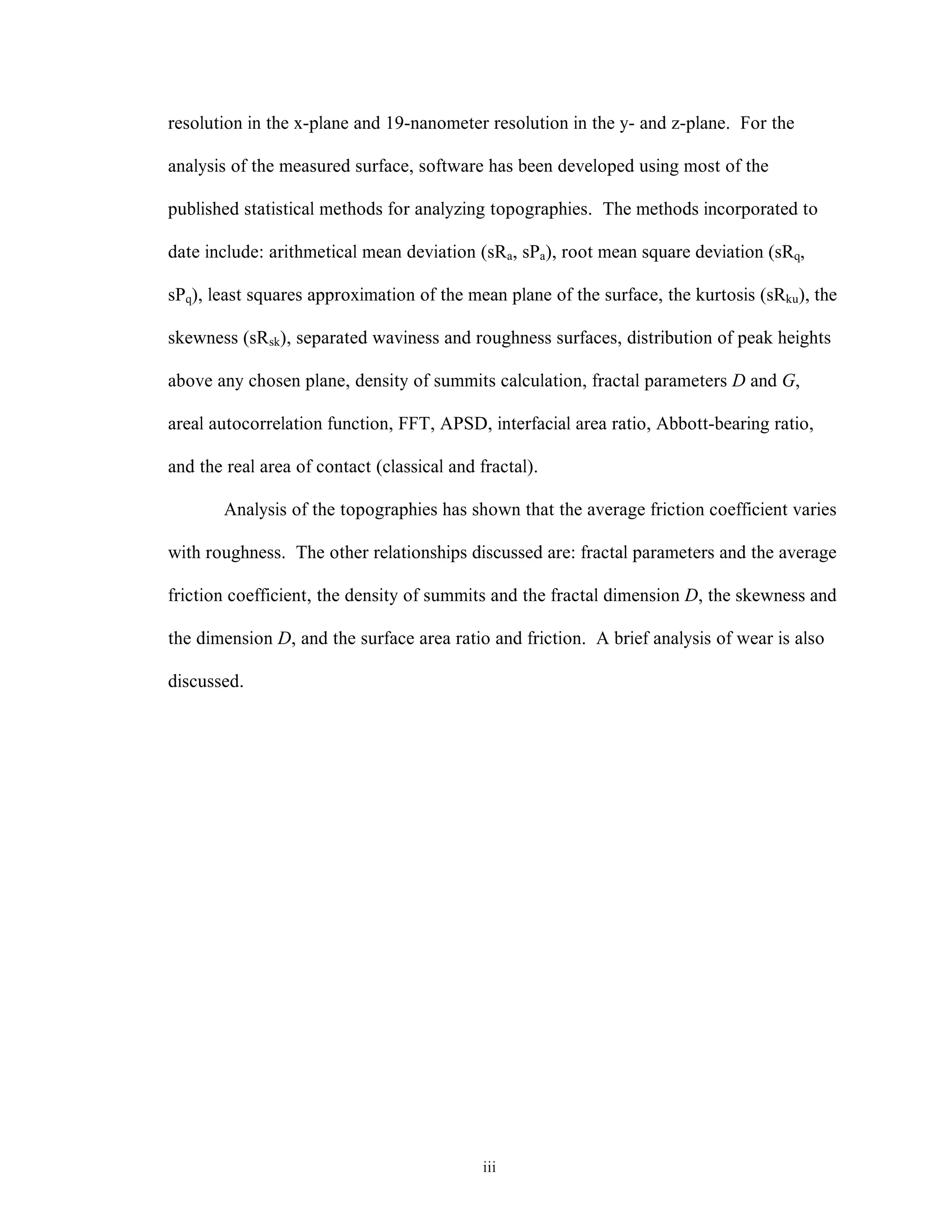
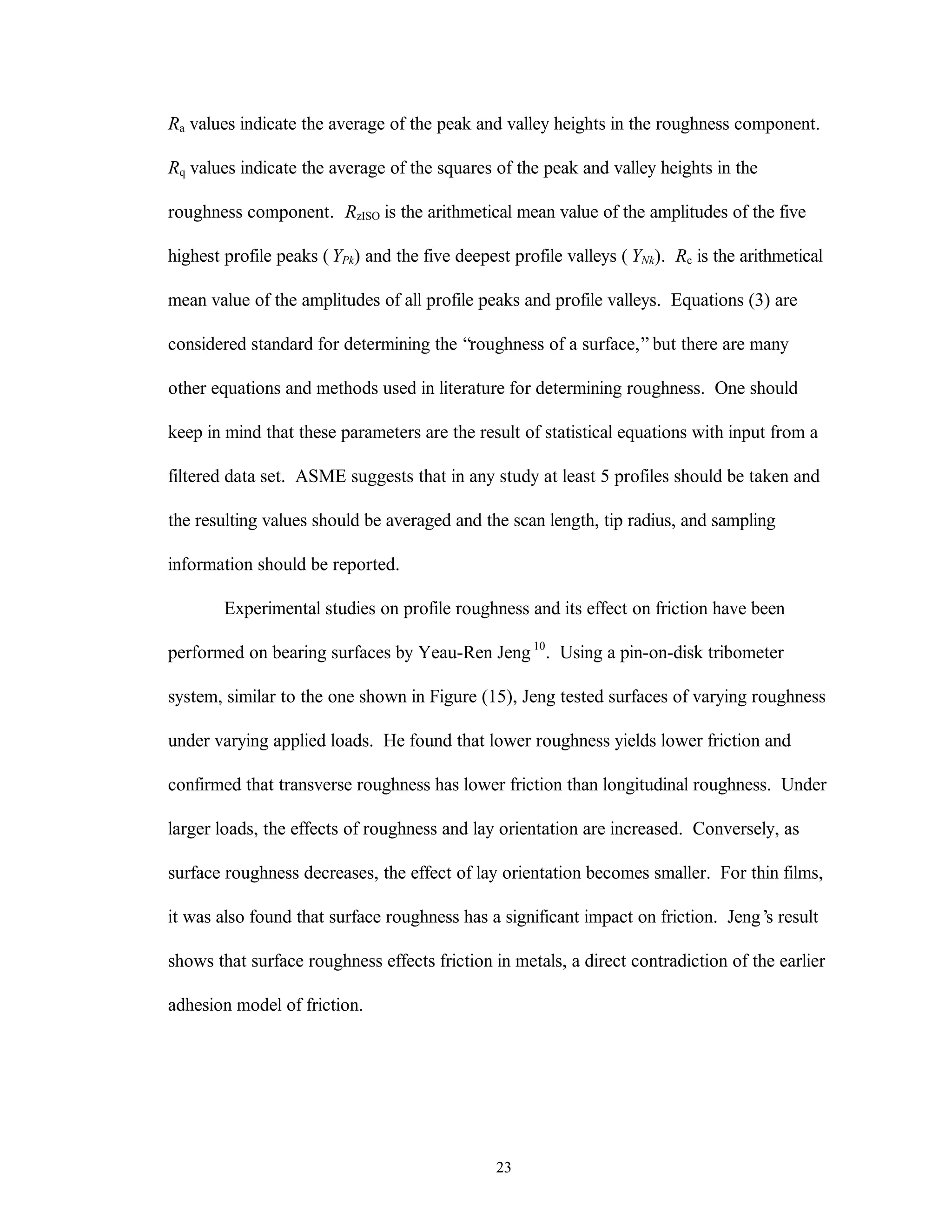
FIG. 15. Pin on disk tribometer made by Micro Photonics [photo from their website at
www.microphotonics.com].
Experimental studies of roughness using single profilometer traces were
abandoned early in the present study because, statistically, a topographical profile will
yield a better population sample than a trace. This results in values that are more
representative of the surface. Marx et al.5
found that for C-C composite materials single
profile roughness intermittently correlated with the measured average friction coefficient
from dynamometer testing.
III. Basic Fractal Theory
Fractal theory was introduced by Benoit B. Mandelbrot11
at the beginning of the
1970’s. Fractals, however, were discovered by mathematicians over a century ago and
have been used as subtle examples of continuous, non-rectifiable curves (those whose
length cannot be measured) or of continuous, non-differentiable curves (those for which it
is impossible to draw a tangent at any of their points). Mandelbrot realized that many](https://image.slidesharecdn.com/8bf0a7f6-6ca6-4e58-84b7-6c9f74012ad7-160219070136/75/TodPmastersthesis-35-2048.jpg)
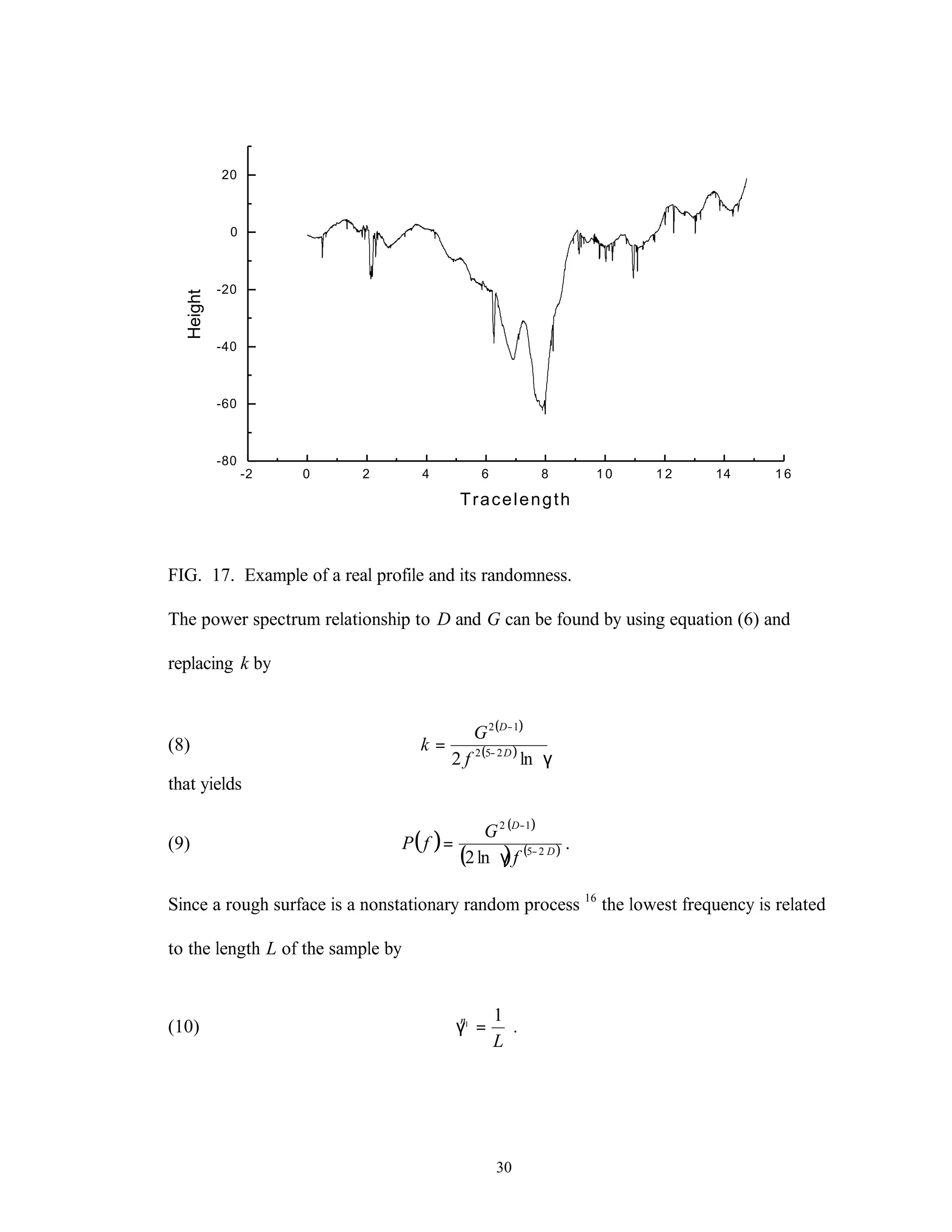
![32
-0.10 -0.05 0.00 0.05 0.10
0
20000
40000
60000
80000
P(f)
f
1E-3 0.01 0.1
100
1000
10000
log[(P(f)]
log [f]
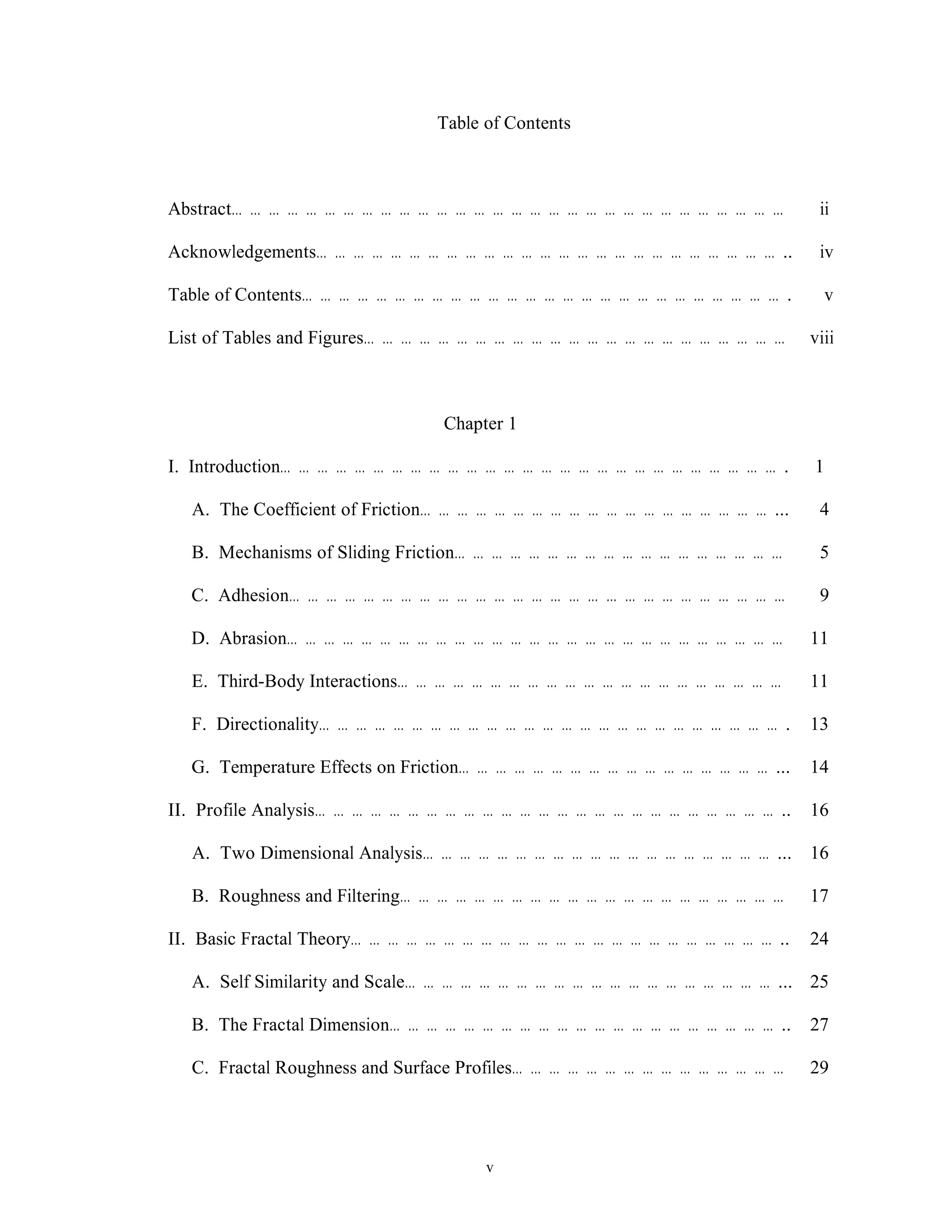
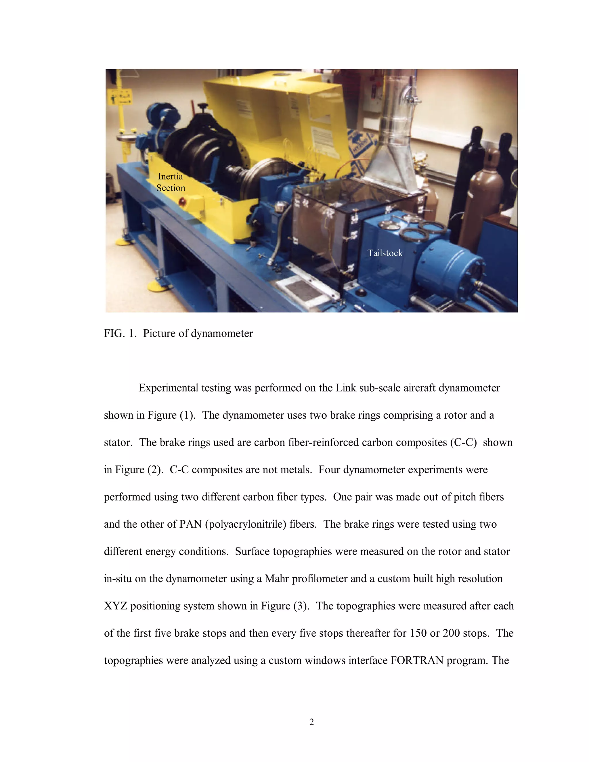
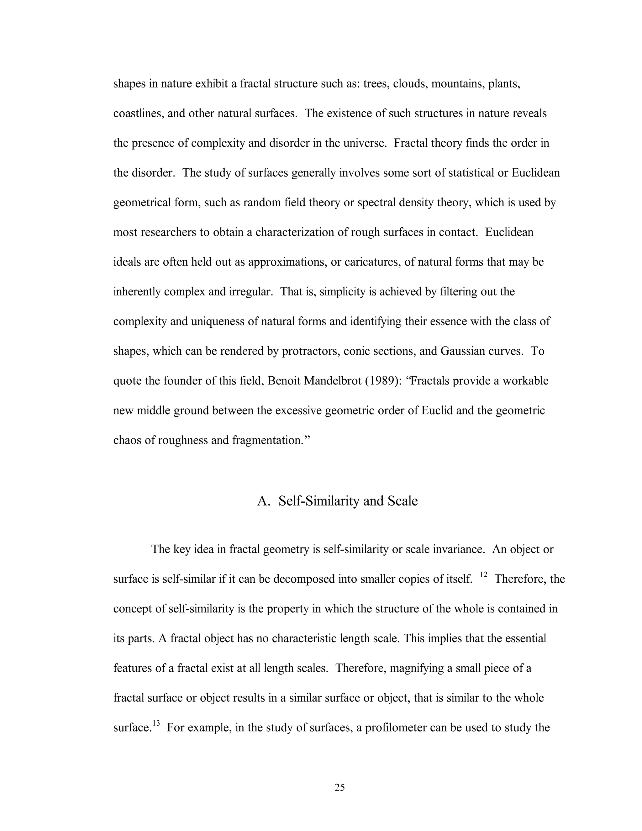
FIG. 19. The power spectrum (left) and log(f) vs. log(p(f)) (right).
If P(f) is plotted as a function of f on a log-log plot as in Figure (19), then the power law
behavior would result in a straight line. The slope of the line η and the topological
dimension d are related to the dimension D as12
(11)
2
3 η−
+= dD .
The topological dimension d for a profile is 1 and for a surface it is 2. To find the
parameter G, D must be calculated first. The idea behind the fractal approach is that
instead of characterizing the actual disorder of surface roughness as the classical statistical
methods do, it is more logical to identify and characterize the order behind the disorder.
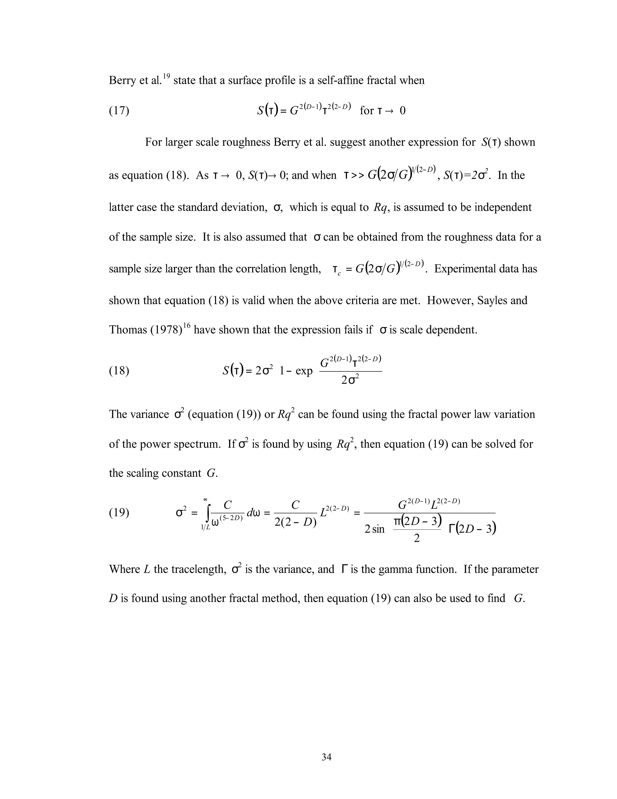
The variance function or structure function (SF) shown as equation (12) 14
, can be
used for the calculation of a measured surface profile with a total of N points. The SF
S(τ) can be calculated by varying the distance τ from a given point z(xi) and then finding
the difference z(xi) –z(xi + τ). The critical value of τ occurs when N = τ/∆x where ∆x is
the sample spacing. The benefit of using the SF is that it prevents aliasing (misplaced](https://image.slidesharecdn.com/8bf0a7f6-6ca6-4e58-84b7-6c9f74012ad7-160219070136/75/TodPmastersthesis-43-2048.jpg)
![33
harmonics) in the power spectrum. 17
Aliasing arises because the roughness profile is not
bandwidth limited to the Nyquist critical frequency ωH. The aliasing causes the power of
frequencies in the range ω > ωH to be falsely translated into the range ω < ωH. By
avoiding aliasing, the structure function yields more accurate values for D and G.14
(12) ( ) ( )[ ]∑
∆
τ−
=
τ+−
∆
τ−
=τ
x
N
i
ii xzxz
x
N
S
1
21
)(
A trace is said to be fractal if the structure function has a power law form: 1
(13) ( ) ( )DD
GS −−
τ=τ 2212
)(
The fractal parameters G and D are found from the power spectrum as mentioned earlier.
Alternatively, equation (13) has been derived from the power spectrum using the relation 18
(14) ( ) ( )[ ]1
1
−ω=τ τω
=
∑ ii
N
i
i ePS
As in the power spectrum method for finding the D and G parameters, the structure
function S(τ) can be plotted against τ on a log-log plot. The curve will be a straight line if
the profile is fractal. The slope of the line is related to D as in equation (11). The value of
G is obtained from the intercept at a certain value of τ. Using the fractal power law of
equation (6) in equation (14), the structure function is then given by 18
(15) ( ) ( ) ( ) ( )D
D
D
D
C
S −
τ−Γ
−π
−
=τ 22
32
2
32
sin
2
where Γ is the gamma function, and the constant C of the power spectrum is related to G
of the structure function as
(16)
( )
( ) ( )32
2
32
sin
2 )1(2
−Γ
−
−
=
−
D
D
GD
C
D
π](https://image.slidesharecdn.com/8bf0a7f6-6ca6-4e58-84b7-6c9f74012ad7-160219070136/75/TodPmastersthesis-44-2048.jpg)

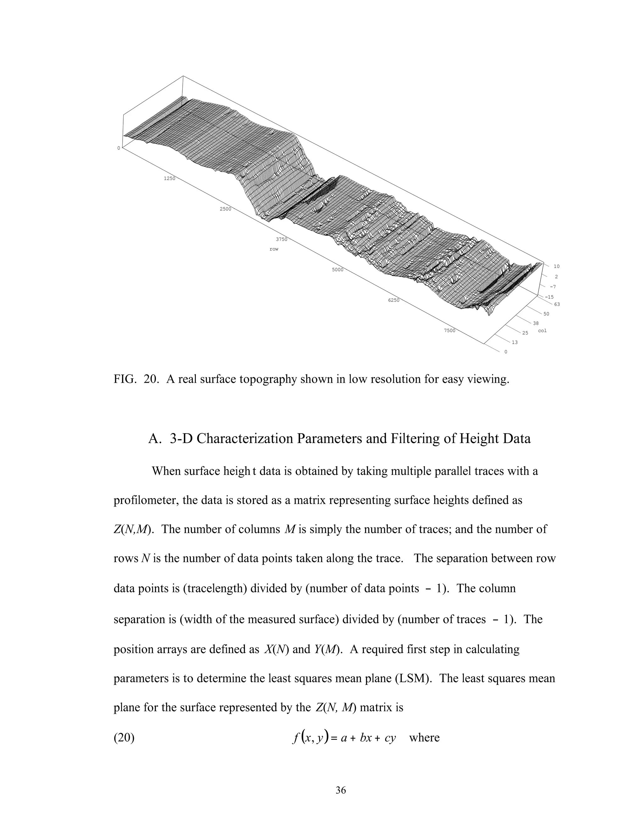
![37
a Z bX cY= − −
( ) ( )[ ]
( ) ( )[ ]
b
X k Z k j Z
X k X k X
j
M
k
N
j
M
k
N
=
−
−
==
==
∑∑
∑∑
,
11
11
( ) ( )[ ]
( ) ( )[ ]
c
Y j Z k j Z
Y j Y j Y
j
M
k
N
j
M
k
N
=
−
−
==
==
∑∑
∑∑
,
11
11
The variables b and c are the slopes in the two orthogonal directions and a is the height
intersecting the Z-axis (or the datum plane). The residual surface R(N,M) can be obtained
by equation (21).
(21) ( ) ( ) ( ) ( )( )R N M Z N M a bX N cY M, ,= − + +
The residual surface R(N, M) can now be used to calculate surface parameters.
Since the separation between rows and columns can be different, a length scale l
must be defined. The length scale at which a surface is measured is important because
some parameters characterizing the surface can change significantly with a change in
scale. This is not true for all parameters though. Let
(22) l l lx y= +
2 2
where lx is the spacing between the rows and ly is the spacing between the columns. The
length scale (hypotenuse) l can be thought of as a magnification of the surface and its
resolution in the surface plane is l units. For fractal calculations l is the asperity base
diameter. The height resolution depends on the measuring instrument. The tip radius of
a stylus used in profilometry is neglected in this study since the length scale is of the
same order of magnitude as the stylus tip radius (2µm - 10µm).](https://image.slidesharecdn.com/8bf0a7f6-6ca6-4e58-84b7-6c9f74012ad7-160219070136/75/TodPmastersthesis-48-2048.jpg)